AGÕæÈË°Ù¼ÒÀÖ¹Ù·½ÍøÕ¾

In this tutorial, we will subset an existing HDF5 file containing NEON hyperspectral data. The purpose of this exercise is to generate a smaller file for use in subsequent analyses to reduce the file transfer time and processing power needed.

Why subset your dataset?

There are many reasons why you may wish to subset your HDF5 file. Primarily, HDF5 files may contain a large amount of information that is not necessary for your purposes. By subsetting the file, you can reduce file size, thereby shrinking your storage needs, shortening file transfer/download times, and reducing your processing time for analysis. In this example, we will take a full HDF5 file of NEON hyperspectral reflectance data from the San Joaquin Experimental Range (SJER) that has a file size of ~652 Mb and make a new HDF5 file with a reduced spatial extent, and a reduced spectral resolution, yielding a file of only ~50.1 Mb. This reduction in file size will make it easier and faster to conduct your analysis and to share your data with others. We will then use this subsetted file in the Introduction to Hyperspectral Remote Sensing Data series.

If you find that downloading the full 652 Mb file takes too much time or storage space, you will find a link to this subsetted file at the top of each lesson in the Introduction to Hyperspectral Remote Sensing Data series.

Exploring the NEON hyperspectral HDF5 file structure

In order to determine what information that we want to put into our subset, we should first take a look at the full NEON hyperspectral HDF5 file structure to see what is included. To do so, we will load the required package for this tutorial (you can un-comment the middle two lines to load 'BiocManager' and 'rhdf5' if you don't already have it on your computer).

# Install rhdf5 package (only need to run if not already installed)
# install.packages("BiocManager")
# BiocManager::install("rhdf5")

# Load required packages
library(rhdf5)

Next, we define our working directory where we have saved the full HDF5 file of NEON hyperspectral reflectance data from the SJER site. Note, the filepath to the working directory will depend on your local environment. Then, we create a string (f) of the HDF5 filename and read its attributes.

# set working directory to ensure R can find the file we wish to import and where
# we want to save our files. Be sure to move the download into your working directory!
wd <- "~/Documents/data/" # This will depend on your local environment
setwd(wd)

# Make the name of our HDF5 file a variable
f_full <- paste0(wd,"NEON_D17_SJER_DP3_257000_4112000_reflectance.h5")

Next, let's take a look at the structure of the full NEON hyperspectral reflectance HDF5 file.

View(h5ls(f_full, all=T))

Wow, there is a lot of information in there! The majority of the groups contained within this file are Metadata, most of which are used for processing the raw observations into the reflectance product that we want to use. For demonstration and teaching purposes, we will not need this information. What we will need are things like the Coordinate_System information (so that we can georeference these data), the Wavelength dataset (so that we can match up each band with its appropriate wavelength in the electromagnetic spectrum), and of course the Reflectance_Data themselves. You can also see that each group and dataset has a number of associated attributes (in the 'num_attrs' column). We will want to copy over those attributes into the data subset as well. But first, we need to define each of the groups that we want to populate in our new HDF5 file.

Create new HDF5 file framework

In order to make a new subset HDF5 file, we first must create an empty file with the appropriate name, then we will begin to fill in that file with the essential data and attributes that we want to include. Note that the function h5createFile() will not overwrite an existing file. Therefore, if you have already created or downloaded this file, the function will throw an error! Each function should return 'TRUE' if it runs correctly.

# First, create a name for the new file
f <- paste0(wd, "NEON_hyperspectral_tutorial_example_subset.h5")

# create hdf5 file
h5createFile(f)

## [1] TRUE

# Now we create the groups that we will use to organize our data
h5createGroup(f, "SJER/")

## [1] TRUE

h5createGroup(f, "SJER/Reflectance")

## [1] TRUE

h5createGroup(f, "SJER/Reflectance/Metadata")

## [1] TRUE

h5createGroup(f, "SJER/Reflectance/Metadata/Coordinate_System")

## [1] TRUE

h5createGroup(f, "SJER/Reflectance/Metadata/Spectral_Data")

## [1] TRUE

Adding group attributes

One of the great things about HDF5 files is that they can contain data and attributes within the same group. As explained within the Introduction to Working with HDF5 Format in R series, attributes are a type of metadata that are associated with an HDF5 group or dataset. There may be multiple attributes associated with each group and/or dataset. Attributes come with a name and an associated array of information. In this tutorial, we will read the existing attribute data from the full hyperspectral tile using the h5readAttributes() function (which returns a list of attributes), then we loop through those attributes and write each attribute to its appropriate group using the h5writeAttribute() function.

First, we will do this for the low-level "SJER/Reflectance" group. In this step, we are adding attributes to a group rather than a dataset. To do so, we must first open a file and group interface using the H5Fopen and H5Gopen functions, then we can use h5writeAttribute() to edit the group that we want to give an attribute.

a <- h5readAttributes(f_full,"/SJER/Reflectance/")
fid <- H5Fopen(f)
g <- H5Gopen(fid, "SJER/Reflectance")

for(i in 1:length(names(a))){
  h5writeAttribute(attr = a[[i]], h5obj=g, name=names(a[i]))
}

# It's always a good idea to close the file connection immidiately
# after finishing each step that leaves an open connection.
h5closeAll()

Next, we will loop through each of the datasets within the Coordinate_System group, and copy those (and their attributes, if present) from the full tile to our subset file. The Coordinate_System group contains many important pieces of information for geolocating our data, so we need to make sure that the subset file has that information.

# make a list of all groups within the full tile file
ls <- h5ls(f_full,all=T)

# make a list of all of the names within the Coordinate_System group
cg <- unique(ls[ls$group=="/SJER/Reflectance/Metadata/Coordinate_System",]$name)

# Loop through the list of datasets that we just made above
for(i in 1:length(cg)){
  print(cg[i])
  
  # Read the inividual dataset within the Coordinate_System group
  d=h5read(f_full,paste0("/SJER/Reflectance/Metadata/Coordinate_System/",cg[i]))

  # Read the associated attributes (if any)
  a=h5readAttributes(f_full,paste0("/SJER/Reflectance/Metadata/Coordinate_System/",cg[i]))
    
  # Assign the attributes (if any) to the dataset
  attributes(d)=a
  
  # Finally, write the dataset to the HDF5 file
  h5write(obj=d,file=f,
          name=paste0("/SJER/Reflectance/Metadata/Coordinate_System/",cg[i]),
          write.attributes=T)
}

## [1] "Coordinate_System_String"
## [1] "EPSG Code"
## [1] "Map_Info"
## [1] "Proj4"

Spectral Subsetting

The goal of subsetting this dataset is to substantially reduce the file size, making it faster to download and process these data. While each AOP mosaic tile is not particularly large in terms of its spatial scale (1km by 1km at 1m resolution= 1,000,000 pixels, or about half as many pixels at shown on a standard 1080p computer screen), the 426 spectral bands available result in a fairly large file size. Therefore, we will reduce the spectral resolution of these data by selecting every fourth band in the dataset, which reduces the file size to 1/4 of the original!

Some circumstances demand the full spectral resolution file. For example, if you wanted to discern between the spectral signatures of similar minerals, or if you were conducting an analysis of the differences in the 'red edge' between plant functional types, you would want to use the full spectral resolution of the original hyperspectral dataset. Still, we can use far fewer bands for demonstration and teaching purposes, while still getting a good sense of what these hyperspectral data can do.

# First, we make our 'index', a list of number that will allow us to select every fourth band, using the "sequence" function seq()
idx <- seq(from = 1, to = 426, by = 4)

# We then use this index to select particular wavelengths from the full tile using the "index=" argument
wavelengths <- h5read(file = f_full, 
             name = "SJER/Reflectance/Metadata/Spectral_Data/Wavelength", 
             index = list(idx)
            )

# As per above, we also need the wavelength attributes
wavelength.attributes <- h5readAttributes(file = f_full, 
                       name = "SJER/Reflectance/Metadata/Spectral_Data/Wavelength")
attributes(wavelengths) <- wavelength.attributes

# Finally, write the subset of wavelengths and their attributes to the subset file
h5write(obj=wavelengths, file=f,
        name="SJER/Reflectance/Metadata/Spectral_Data/Wavelength",
        write.attributes=T)

Spatial Subsetting

Even after spectral subsetting, our file size would be greater than 100Mb. herefore, we will also perform a spatial subsetting process to further reduce our file size. Now, we need to figure out which part of the full image that we want to extract for our subset. It takes a number of steps in order to read in a band of data and plot the reflectance values - all of which are thoroughly described in the Intro to Working with Hyperspectral Remote Sensing Data in HDF5 Format in R tutorial. For now, let's focus on the essentials for our problem at hand. In order to explore the spatial qualities of this dataset, let's plot a single band as an overview map to see what objects and land cover types are contained within this mosaic tile. The Reflectance_Data dataset has three dimensions in the order of bands, columns, rows. We want to extract a single band, and all 1,000 columns and rows, so we will feed those values into the index= argument as a list. For this example, we will select the 58th band in the hyperspectral dataset, which corresponds to a wavelength of 667nm, which is in the red end of the visible electromagnetic spectrum. We will use NULL in the column and row position to indicate that we want all of the columns and rows (we agree that it is weird that NULL indicates "all" in this circumstance, but that is the default behavior for this, and many other, functions).

# Extract or "slice" data for band 58 from the HDF5 file
b58 <- h5read(f_full,name = "SJER/Reflectance/Reflectance_Data",
             index=list(58,NULL,NULL))
h5closeAll()

# convert from array to matrix
b58 <- b58[1,,]

# Make a plot to view this band
image(log(b58), col=grey(0:100/100))

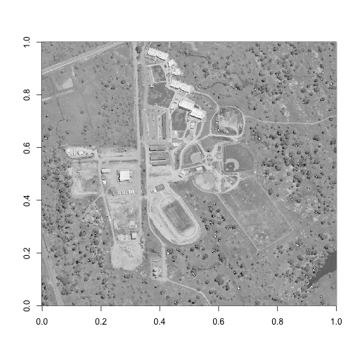
As we can see here, this hyperspectral reflectance tile contains a school campus that is under construction. There are many different land cover types contained here, which makes it a great example! Perhaps the most unique feature shown is in the bottom right corner of this image, where we can see the tip of a small reservoir. Let's be sure to capture this feature in our spatial subset, as well as a few other land cover types (irrigated grass, trees, bare soil, and buildings).

While raster images count their pixels from the top left corner, we are working with a matrix, which counts its pixels from the bottom left corner. Therefore, rows are counted from the bottom to the top, and columns are counted from the left to the right. If we want to sample the bottom right quadrant of this image, we need to select rows 1 through 500 (bottom half), and columns 501 through 1000 (right half). Note that, as above, the index= argument in h5read() requires a list of three dimensions for this example - in the order of bands, columns, rows.

subset_rows <- 1:500
subset_columns <- 501:1000
# Extract or "slice" data for band 44 from the HDF5 file
b58 <- h5read(f_full,name = "SJER/Reflectance/Reflectance_Data",
             index=list(58,subset_columns,subset_rows))
h5closeAll()

# convert from array to matrix
b58 <- b58[1,,]

# Make a plot to view this band
image(log(b58), col=grey(0:100/100))

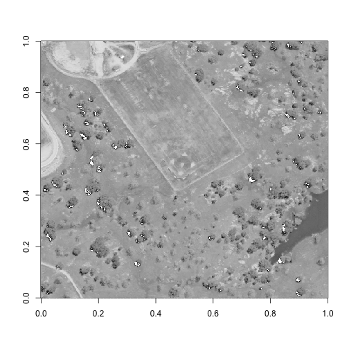
Perfect - now we have a spatial subset that includes all of the different land cover types that we are interested in investigating.

Extracting a subset

Now that we have determined our ideal spectral and spatial subsets for our analysis, we are ready to put both of those pieces of information into our h5read() function to extract our example subset out of the full NEON hyperspectral dataset. Here, we are taking every fourth band (using our idx variabe), columns 501:1000 (the right half of the tile) and rows 1:500 (the bottom half of the tile). The results in us extracting every fourth band of the bottom-right quadrant of the mosaic tile.

# Read in reflectance data.
# Note the list that we feed into the index argument! 
# This tells the h5read() function which bands, rows, and 
# columns to read. This is ultimately how we reduce the file size.
hs <- h5read(file = f_full, 
             name = "SJER/Reflectance/Reflectance_Data", 
             index = list(idx, subset_columns, subset_rows)
            )

As per the 'adding group attributes' section above, we will need to add the attributes to the hyperspectral data (hs) before writing to the new HDF5 subset file (f). The hs variable already has one attribute, $dim, which contains the actual dimensions of the hs array, and will be important for writing the array to the f file later. We will want to combine this attribute with all of the other Reflectance_Data group attributes from the original HDF5 file, f. However, some of the attributes will no longer be valid, such as the Dimensions and Spatial_Extent_meters attributes, so we will need to overwrite those before assigning these attributes to the hs variable to then write to the f file.

# grab the '$dim' attribute - as this will be needed 
# when writing the file at the bottom
hsd <- attributes(hs)

# We also need the attributes for the reflectance data.
ha <- h5readAttributes(file = f_full, 
                       name = "SJER/Reflectance/Reflectance_Data")

# However, some of the attributes are not longer valid since 
# we changed the spatial extend of this dataset. therefore, 
# we will need to overwrite those with the correct values.
ha$Dimensions <- c(500,500,107) # Note that the HDF5 file saves dimensions in a different order than R reads them
ha$Spatial_Extent_meters[1] <- ha$Spatial_Extent_meters[1]+500
ha$Spatial_Extent_meters[3] <- ha$Spatial_Extent_meters[3]+500
attributes(hs) <- c(hsd,ha)

# View the combined attributes to ensure they are correct
attributes(hs)

## $dim
## [1] 107 500 500
## 
## $Cloud_conditions
## [1] "For cloud conditions information see Weather Quality Index dataset."
## 
## $Cloud_type
## [1] "Cloud type may have been selected from multiple flight trajectories."
## 
## $Data_Ignore_Value
## [1] -9999
## 
## $Description
## [1] "Atmospherically corrected reflectance."
## 
## $Dimension_Labels
## [1] "Line, Sample, Wavelength"
## 
## $Dimensions
## [1] 500 500 107
## 
## $Interleave
## [1] "BSQ"
## 
## $Scale_Factor
## [1] 10000
## 
## $Spatial_Extent_meters
## [1]  257500  258000 4112500 4113000
## 
## $Spatial_Resolution_X_Y
## [1] 1 1
## 
## $Units
## [1] "Unitless."
## 
## $Units_Valid_range
## [1]     0 10000

# Finally, write the hyperspectral data, plus attributes, 
# to our new file 'f'.
h5write(obj=hs, file=f,
        name="SJER/Reflectance/Reflectance_Data",
        write.attributes=T)

## You created a large dataset with compression and chunking.
## The chunk size is equal to the dataset dimensions.
## If you want to read subsets of the dataset, you should testsmaller chunk sizes to improve read times.

# It's always a good idea to close the HDF5 file connection
# before moving on.
h5closeAll()

That's it! We just created a subset of the original HDF5 file, and included the most essential groups and metadata for exploratory analysis. You may consider adding other information, such as the weather quality indicator, when subsetting datasets for your own purposes.

If you want to take a look at the subset that you just made, run the h5ls() function:

View(h5ls(f, all=T))