AGÕæÈË°Ù¼ÒÀÖ¹Ù·½ÍøÕ¾

This activity will walk you through the fundamental principles of working with raster data in R.

What is Raster Data?

Raster or "gridded" data are data that are saved in pixels. In the spatial world, each pixel represents an area on the Earth's surface. For example in the raster below, each pixel represents a particular land cover class that would be found in that location in the real world.

More on rasters in the The Relationship Between Raster Resolution, Spatial extent & Number of Pixels tutorial.

To work with rasters in R, we need two key packages, sp and raster. To install the raster package you can use install.packages('raster'). When you install the raster package, sp should also install. Also install the rgdal package install.packages('rgdal'). Among other things, rgdal will allow us to export rasters to GeoTIFF format.

Once installed we can load the packages and start working with raster data.

# load the raster, sp, and rgdal packages
library(raster)
library(sp)
library(rgdal)

# set working directory to data folder
#setwd("pathToDirHere")
wd <- ("~/Git/data/")
setwd(wd)

Next, let's load a raster containing elevation data into our environment. And look at the attributes.

# load raster in an R object called 'DEM'
DEM <- raster(paste0(wd, "NEON-DS-Field-Site-Spatial-Data/SJER/DigitalTerrainModel/SJER2013_DTM.tif"))

# look at the raster attributes. 
DEM

## class      : RasterLayer 
## dimensions : 5060, 4299, 21752940  (nrow, ncol, ncell)
## resolution : 1, 1  (x, y)
## extent     : 254570, 258869, 4107302, 4112362  (xmin, xmax, ymin, ymax)
## crs        : +proj=utm +zone=11 +datum=WGS84 +units=m +no_defs 
## source     : /Users/olearyd/Git/data/NEON-DS-Field-Site-Spatial-Data/SJER/DigitalTerrainModel/SJER2013_DTM.tif 
## names      : SJER2013_DTM

Notice a few things about this raster.

• dimensions: the "size" of the file in pixels

• nrow, ncol: the number of rows and columns in the data (imagine a spreadsheet or a matrix).
• ncells: the total number of pixels or cells that make up the raster.

• resolution: the size of each pixel (in meters in this case). 1 meter pixels means that each pixel represents a 1m x 1m area on the earth's surface.
• extent: the spatial extent of the raster. This value will be in the same coordinate units as the coordinate reference system of the raster.
• coord ref: the coordinate reference system string for the raster. This raster is in UTM (Universal Trans Mercator) zone 11 with a datum of WGS 84. .

Work with Rasters in R

Now that we have the raster loaded into R, let's grab some key raster attributes.

Define Min/Max Values

By default this raster doesn't have the min or max values associated with it's attributes Let's change that by using the setMinMax() function.

# calculate and save the min and max values of the raster to the raster object
DEM <- setMinMax(DEM)

# view raster attributes
DEM

## class      : RasterLayer 
## dimensions : 5060, 4299, 21752940  (nrow, ncol, ncell)
## resolution : 1, 1  (x, y)
## extent     : 254570, 258869, 4107302, 4112362  (xmin, xmax, ymin, ymax)
## crs        : +proj=utm +zone=11 +datum=WGS84 +units=m +no_defs 
## source     : /Users/olearyd/Git/data/NEON-DS-Field-Site-Spatial-Data/SJER/DigitalTerrainModel/SJER2013_DTM.tif 
## names      : SJER2013_DTM 
## values     : 228.1, 518.66  (min, max)

Notice the values is now part of the attributes and shows the min and max values for the pixels in the raster. What these min and max values represent depends on what is represented by each pixel in the raster.

You can also view the rasters min and max values and the range of values contained within the pixels.

#Get min and max cell values from raster
#NOTE: this code may fail if the raster is too large
cellStats(DEM, min)

## [1] 228.1

cellStats(DEM, max)

## [1] 518.66

cellStats(DEM, range)

## [1] 228.10 518.66

View CRS

First, let's consider the Coordinate Reference System (CRS).

#view coordinate reference system
DEM@crs

## CRS arguments:
##  +proj=utm +zone=11 +datum=WGS84 +units=m +no_defs

This raster is located in UTM Zone 11.

View Extent

If you want to know the exact boundaries of your raster that is in the extent slot.

# view raster extent
DEM@extent

## class      : Extent 
## xmin       : 254570 
## xmax       : 258869 
## ymin       : 4107302 
## ymax       : 4112362

Raster Pixel Values

We can also create a histogram to view the distribution of values in our raster. Note that the max number of pixels that R will plot by default is 100,000. We can tell it to plot more using the maxpixels attribute. Be careful with this, if your raster is large this can take a long time or crash your program.

Since our raster is a digital elevation model, we know that each pixel contains elevation data about our area of interest. In this case the units are meters.

This is an easy and quick data checking tool. Are there any totally weird values?

# the distribution of values in the raster
hist(DEM, main="Distribution of elevation values", 
     col= "purple", 
     maxpixels=22000000)

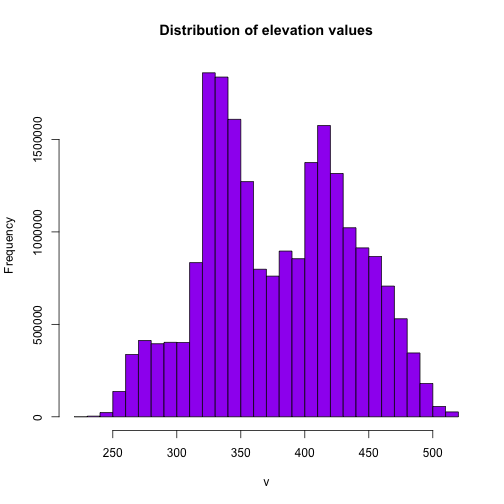
It looks like we have a lot of land around 325m and 425m.

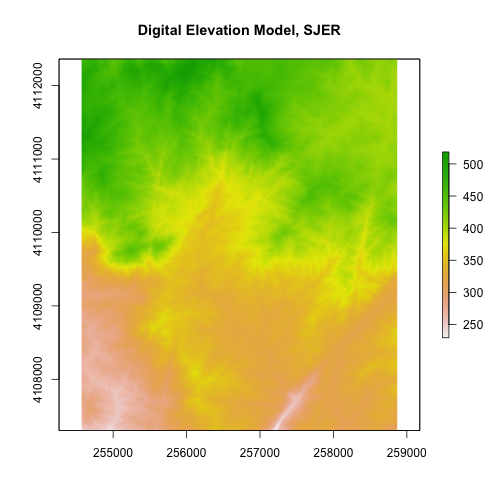
Plot Raster Data

Let's take a look at our raster now that we know a bit more about it. We can do a simple plot with the plot() function.

# plot the raster
# note that this raster represents a small region of the NEON SJER field site
plot(DEM, 
		 main="Digital Elevation Model, SJER") # add title with main

R has an image() function that allows you to control the way a raster is rendered on the screen. The plot() function in R has a base setting for the number of pixels that it will plot (100,000 pixels). The image command thus might be better for rendering larger rasters.

# create a plot of our raster
image(DEM)

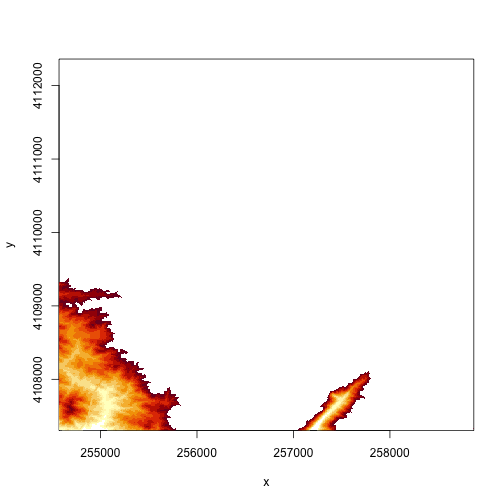
# specify the range of values that you want to plot in the DEM
# just plot pixels between 250 and 300 m in elevation
image(DEM, zlim=c(250,300))

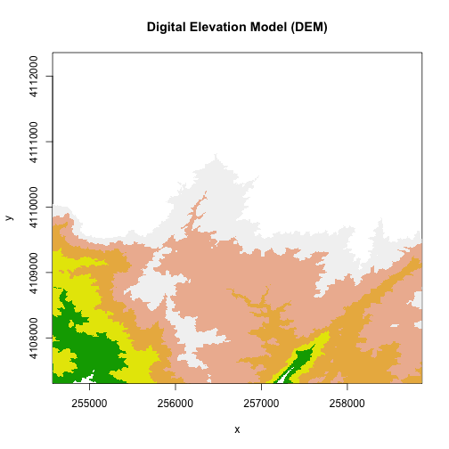
# we can specify the colors too
col <- terrain.colors(5)
image(DEM, zlim=c(250,375), main="Digital Elevation Model (DEM)", col=col)

Plotting with Colors

In the above example. terrain.colors() tells R to create a palette of colors within the terrain.colors color ramp. There are other palettes that you can use as well include rainbow and heat.colors.

Breaks and Colorbars in R

A digital elevation model (DEM) is an example of a continuous raster. It contains elevation values for a range. For example, elevations values in a DEM might include any set of values between 200 m and 500 m. Given this range, you can plot DEM pixels using a gradient of colors.

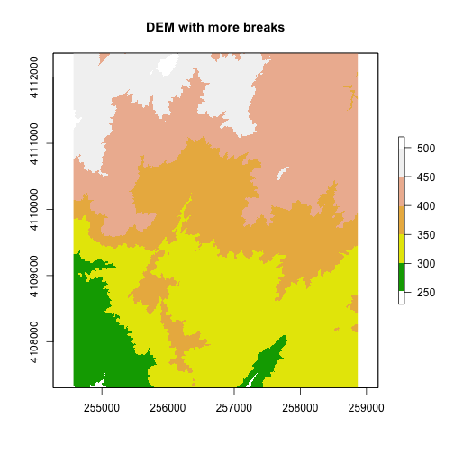
By default, R will assign the gradient of colors uniformly across the full range of values in the data. In our case, our DEM has values between 250 and 500. However, we can adjust the "breaks" which represent the numeric locations where the colors change if we want too.

# add a color map with 5 colors
col=terrain.colors(5)

# add breaks to the colormap (6 breaks = 5 segments)
brk <- c(250, 300, 350, 400, 450, 500)

plot(DEM, col=col, breaks=brk, main="DEM with more breaks")

We can also customize the legend appearance.

# First, expand right side of clipping rectangle to make room for the legend
# turn xpd off
par(xpd = FALSE, mar=c(5.1, 4.1, 4.1, 4.5))

# Second, plot w/ no legend
plot(DEM, col=col, breaks=brk, main="DEM with a Custom (but flipped) Legend", legend = FALSE)

# Third, turn xpd back on to force the legend to fit next to the plot.
par(xpd = TRUE)

# Fourth, add a legend - & make it appear outside of the plot
legend(par()$usr[2], 4110600,
        legend = c("lowest", "a bit higher", "middle ground", "higher yet", "highest"), 
        fill = col)

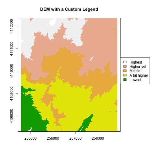
Notice that the legend is in reverse order in the previous plot. Let’s fix that. We need to both reverse the order we have the legend laid out and reverse the the color fill with the rev() colors.

# Expand right side of clipping rect to make room for the legend
par(xpd = FALSE,mar=c(5.1, 4.1, 4.1, 4.5))
#DEM with a custom legend
plot(DEM, col=col, breaks=brk, main="DEM with a Custom Legend",legend = FALSE)
#turn xpd back on to force the legend to fit next to the plot.
par(xpd = TRUE)

#add a legend - but make it appear outside of the plot
legend( par()$usr[2], 4110600,
        legend = c("Highest", "Higher yet", "Middle","A bit higher", "Lowest"), 
        fill = rev(col))

Try the code again but only make one of the changes -- reverse order or reverse colors-- what happens?

The raster plot now inverts the elevations! This is a good reason to understand your data so that a simple visualization error doesn't have you reversing the slope or some other error.

We can add a custom color map with fewer breaks as well.

#add a color map with 4 colors
col=terrain.colors(4)
#add breaks to the colormap (6 breaks = 5 segments)
brk <- c(200, 300, 350, 400,500)
plot(DEM, col=col, breaks=brk, main="DEM with fewer breaks")

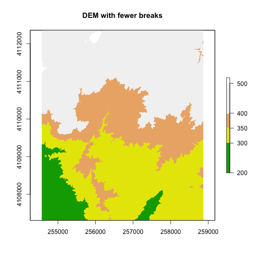
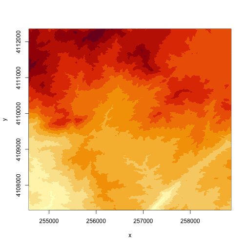
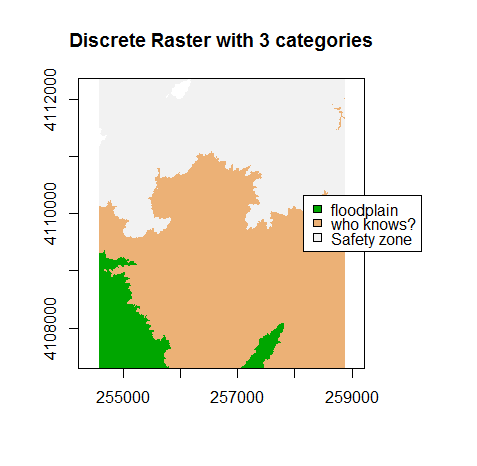
A discrete dataset has a set of unique categories or classes. One example could be land use classes. The example below shows elevation zones generated using the same DEM.

Basic Raster Math

We can also perform calculations on our raster. For instance, we could multiply all values within the raster by 2.

#multiple each pixel in the raster by 2
DEM2 <- DEM * 2

DEM2

## class      : RasterLayer 
## dimensions : 5060, 4299, 21752940  (nrow, ncol, ncell)
## resolution : 1, 1  (x, y)
## extent     : 254570, 258869, 4107302, 4112362  (xmin, xmax, ymin, ymax)
## crs        : +proj=utm +zone=11 +datum=WGS84 +units=m +no_defs 
## source     : memory
## names      : SJER2013_DTM 
## values     : 456.2, 1037.32  (min, max)

#plot the new DEM
plot(DEM2, main="DEM with all values doubled")

Cropping Rasters in R

You can crop rasters in R using different methods. You can crop the raster directly drawing a box in the plot area. To do this, first plot the raster. Then define the crop extent by clicking twice:

1. Click in the UPPER LEFT hand corner where you want the crop box to begin.
2. Click again in the LOWER RIGHT hand corner to define where the box ends.

You'll see a red box on the plot. NOTE that this is a manual process that can be used to quickly define a crop extent.

#plot the DEM
plot(DEM)

#Define the extent of the crop by clicking on the plot
cropbox1 <- drawExtent()

#crop the raster, then plot the new cropped raster
DEMcrop1 <- crop(DEM, cropbox1)

#plot the cropped extent
plot(DEMcrop1)

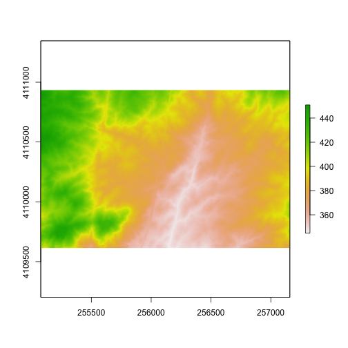
You can also manually assign the extent coordinates to be used to crop a raster. We'll need the extent defined as (xmin, xmax, ymin , ymax) to do this. This is how we'd crop using a GIS shapefile (with a rectangular shape)

#define the crop extent
cropbox2 <-c(255077.3,257158.6,4109614,4110934)
#crop the raster
DEMcrop2 <- crop(DEM, cropbox2)
#plot cropped DEM
plot(DEMcrop2)

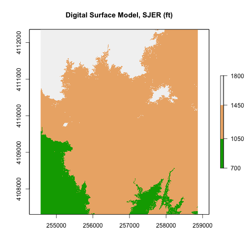
Image (RGB) Data in R

Go to our tutorial Image Raster Data in R - An Intro to learn more about working with image formatted rasters in R.