AGÕæÈË°Ù¼ÒÀÖ¹Ù·½ÍøÕ¾

This tutorial discusses ways to plot plant phenology (discrete time series) and single-aspirated temperature (continuous time series) together. It uses data frames created in the first two parts of this series, Work with NEON OS & IS Data - Plant Phenology & Temperature. If you have not completed these tutorials, please download the dataset below.

To start, we need to set up our R environment. If you're continuing from the previous tutorial in this series, you'll only need to load the new packages.

# Install needed package (only uncomment & run if not already installed)
#install.packages("dplyr")
#install.packages("ggplot2")
#install.packages("scales")

# Load required libraries
library(ggplot2)
library(dplyr)

## 
## Attaching package: 'dplyr'

## The following objects are masked from 'package:stats':
## 
##     filter, lag

## The following objects are masked from 'package:base':
## 
##     intersect, setdiff, setequal, union

library(gridExtra)

## 
## Attaching package: 'gridExtra'

## The following object is masked from 'package:dplyr':
## 
##     combine

library(scales)

options(stringsAsFactors=F) #keep strings as character type not factors

# set working directory to ensure R can find the file we wish to import and where
# we want to save our files. Be sure to move the download into your working directory!
wd <- "~/Documents/data/" # Change this to match your local environment
setwd(wd)

If you don't already have the R objects, temp_day and phe_1sp_2018, loaded you'll need to load and format those data. If you do, you can skip this code.

# Read in data -> if in series this is unnecessary
temp_day <- read.csv(paste0(wd,'NEON-pheno-temp-timeseries/NEONsaat_daily_SCBI_2018.csv'))

phe_1sp_2018 <- read.csv(paste0(wd,'NEON-pheno-temp-timeseries/NEONpheno_LITU_Leaves_SCBI_2018.csv'))

# Convert dates
temp_day$Date <- as.Date(temp_day$Date)
# use dateStat - the date the phenophase status was recorded
phe_1sp_2018$dateStat <- as.Date(phe_1sp_2018$dateStat)

Separate Plots, Same Panel

In this dataset, we have phenology and temperature data from the Smithsonian Conservation Biology Institute (SCBI) NEON field site. There are a variety of ways we may want to look at this data, including aggregated at the site level, by a single plot, or viewing all plots at the same time but in separate plots. In the Work With NEON's Plant Phenology Data and the Work with NEON's Single-Aspirated Air Temperature Data tutorials, we created separate plots of the number of individuals who had leaves at different times of the year and the temperature in 2018.

However, plot the data next to each other to aid comparisons. The grid.arrange() function from the gridExtra package can help us do this.

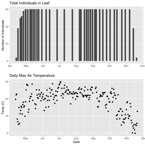
# first, create one plot 
phenoPlot <- ggplot(phe_1sp_2018, aes(dateStat, countYes)) +
    geom_bar(stat="identity", na.rm = TRUE) +
    ggtitle("Total Individuals in Leaf") +
    xlab("") + ylab("Number of Individuals")

# create second plot of interest
tempPlot_dayMax <- ggplot(temp_day, aes(Date, dayMax)) +
    geom_point() +
    ggtitle("Daily Max Air Temperature") +
    xlab("Date") + ylab("Temp (C)")

# Then arrange the plots - this can be done with >2 plots as well.
grid.arrange(phenoPlot, tempPlot_dayMax) 

Now, we can see both plots in the same window. But, hmmm... the x-axis on both plots is kinda wonky. We want the same spacing in the scale across the year (e.g., July in one should line up with July in the other) plus we want the dates to display in the same format(e.g. 2016-07 vs. Jul vs Jul 2018).

Format Dates in Axis Labels

The date format parameter can be adjusted with scale_x_date. Let's format the x-axis ticks so they read "month" (%b) in both graphs. We will use the syntax:

scale_x_date(labels=date_format("%b"")

Rather than re-coding the entire plot, we can add the scale_x_date element to the plot object phenoPlot we just created.

# format x-axis: dates
phenoPlot <- phenoPlot + 
  (scale_x_date(breaks = date_breaks("1 month"), labels = date_format("%b")))

tempPlot_dayMax <- tempPlot_dayMax +
  (scale_x_date(breaks = date_breaks("1 month"), labels = date_format("%b")))

# New plot. 
grid.arrange(phenoPlot, tempPlot_dayMax) 

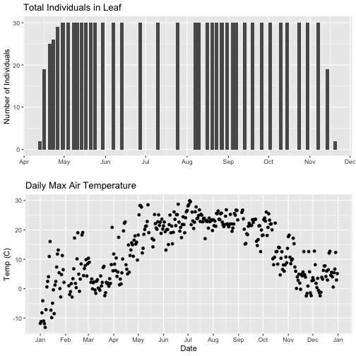
But this only solves one of the problems, we still have a different range on the x-axis which makes it harder to see trends.

Align data sets with different start dates

Now let's work to align the values on the x-axis. We can do this in two ways,

1. setting the x-axis to have the same date range or 2) by filtering the dataset itself to only include the overlapping data. Depending on what you are trying to demonstrate and if you're doing additional analyses and want only the overlapping data, you may prefer one over the other. Let's try both.

Set range of x-axis

Alternatively, we can set the x-axis range for both plots by adding the limits parameter to the scale_x_date() function.

# first, lets recreate the full plot and add in the 
phenoPlot_setX <- ggplot(phe_1sp_2018, aes(dateStat, countYes)) +
    geom_bar(stat="identity", na.rm = TRUE) +
    ggtitle("Total Individuals in Leaf") +
    xlab("") + ylab("Number of Individuals") +
    scale_x_date(breaks = date_breaks("1 month"), 
                  labels = date_format("%b"),
                  limits = as.Date(c('2018-01-01','2018-12-31')))

# create second plot of interest
tempPlot_dayMax_setX <- ggplot(temp_day, aes(Date, dayMax)) +
    geom_point() +
    ggtitle("Daily Max Air Temperature") +
    xlab("Date") + ylab("Temp (C)") +
    scale_x_date(date_breaks = "1 month", 
                 labels=date_format("%b"),
                  limits = as.Date(c('2018-01-01','2018-12-31')))

# Plot
grid.arrange(phenoPlot_setX, tempPlot_dayMax_setX) 

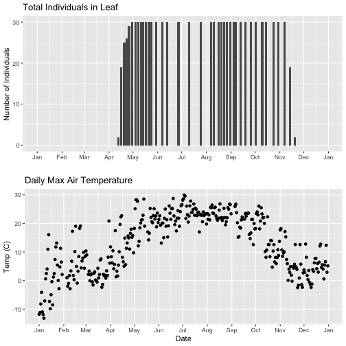
Now we can really see the pattern over the full year. This emphasizes the point that during much of the late fall, winter, and early spring none of the trees have leaves on them (or that data were not collected - this plot would not distinguish between the two).

Subset one data set to match other

Alternatively, we can simply filter the dataset with the larger date range so the we only plot the data from the overlapping dates.

# filter to only having overlapping data
temp_day_filt <- filter(temp_day, Date >= min(phe_1sp_2018$dateStat) & 
                         Date <= max(phe_1sp_2018$dateStat))

# Check 
range(phe_1sp_2018$date)

## [1] "2018-04-13" "2018-11-20"

range(temp_day_filt$Date)

## [1] "2018-04-13" "2018-11-20"

#plot again
tempPlot_dayMaxFiltered <- ggplot(temp_day_filt, aes(Date, dayMax)) +
    geom_point() +
    scale_x_date(breaks = date_breaks("months"), labels = date_format("%b")) +
    ggtitle("Daily Max Air Temperature") +
    xlab("Date") + ylab("Temp (C)")


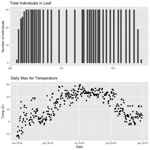
grid.arrange(phenoPlot, tempPlot_dayMaxFiltered)

With this plot, we really look at the area of overlap in the plotted data (but this does cut out the time where the data are collected but not plotted).

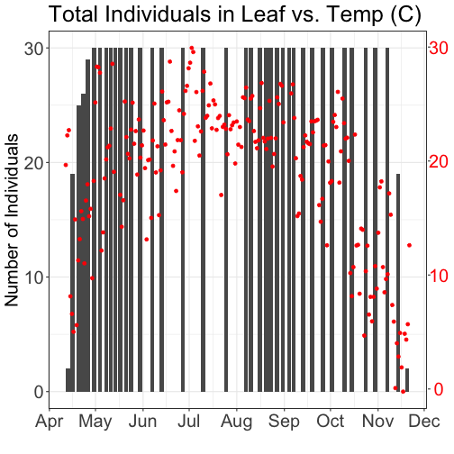
Same plot with two Y-axes

What about layering these plots and having two y-axes (right and left) that have the different scale bars?

Some argue that you should not do this as it can distort what is actually going on with the data. The author of the ggplot2 package is one of these individuals. Therefore, you cannot use ggplot() to create a single plot with multiple y-axis scales. You can read his own discussion of the topic on this .

However, individuals have found work arounds for these plots. The code below is provided as a demonstration of this capability. Note, by showing this code here, we don't necessarily endorse having plots with two y-axes.

This code is adapted from code by .

# Source: http://heareresearch.blogspot.com/2014/10/10-30-2014-dual-y-axis-graph-ggplot2_30.html

# Additional packages needed
library(gtable)
library(grid)


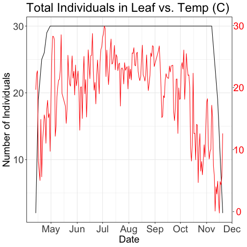
# Plot 1: Pheno data as bars, temp as scatter
grid.newpage()
phenoPlot_2 <- ggplot(phe_1sp_2018, aes(dateStat, countYes)) +
  geom_bar(stat="identity", na.rm = TRUE) +
  scale_x_date(breaks = date_breaks("1 month"), labels = date_format("%b")) +
  ggtitle("Total Individuals in Leaf vs. Temp (C)") +
  xlab(" ") + ylab("Number of Individuals") +
  theme_bw()+
  theme(legend.justification=c(0,1),
        legend.position=c(0,1),
        plot.title=element_text(size=25,vjust=1),
        axis.text.x=element_text(size=20),
        axis.text.y=element_text(size=20),
        axis.title.x=element_text(size=20),
        axis.title.y=element_text(size=20))


tempPlot_dayMax_corr_2 <- ggplot() +
  geom_point(data = temp_day_filt, aes(Date, dayMax),color="red") +
  scale_x_date(breaks = date_breaks("months"), labels = date_format("%b")) +
  xlab("") + ylab("Temp (C)") +
  theme_bw() %+replace% 
  theme(panel.background = element_rect(fill = NA),
        panel.grid.major.x=element_blank(),
        panel.grid.minor.x=element_blank(),
        panel.grid.major.y=element_blank(),
        panel.grid.minor.y=element_blank(),
        axis.text.y=element_text(size=20,color="red"),
        axis.title.y=element_text(size=20))

g1<-ggplot_gtable(ggplot_build(phenoPlot_2))
g2<-ggplot_gtable(ggplot_build(tempPlot_dayMax_corr_2))

pp<-c(subset(g1$layout,name=="panel",se=t:r))
g<-gtable_add_grob(g1, g2$grobs[[which(g2$layout$name=="panel")]],pp$t,pp$l,pp$b,pp$l)

ia<-which(g2$layout$name=="axis-l")
ga <- g2$grobs[[ia]]
ax <- ga$children[[2]]
ax$widths <- rev(ax$widths)
ax$grobs <- rev(ax$grobs)
ax$grobs[[1]]$x <- ax$grobs[[1]]$x - unit(1, "npc") + unit(0.15, "cm")
g <- gtable_add_cols(g, g2$widths[g2$layout[ia, ]$l], length(g$widths) - 1)
g <- gtable_add_grob(g, ax, pp$t, length(g$widths) - 1, pp$b)

grid.draw(g)

# Plot 2: Both pheno data and temp data as line graphs
grid.newpage()
phenoPlot_3 <- ggplot(phe_1sp_2018, aes(dateStat, countYes)) +
  geom_line(na.rm = TRUE) +
  scale_x_date(breaks = date_breaks("months"), labels = date_format("%b")) +
  ggtitle("Total Individuals in Leaf vs. Temp (C)") +
  xlab("Date") + ylab("Number of Individuals") +
  theme_bw()+
  theme(legend.justification=c(0,1),
        legend.position=c(0,1),
        plot.title=element_text(size=25,vjust=1),
        axis.text.x=element_text(size=20),
        axis.text.y=element_text(size=20),
        axis.title.x=element_text(size=20),
        axis.title.y=element_text(size=20))

tempPlot_dayMax_corr_3 <- ggplot() +
  geom_line(data = temp_day_filt, aes(Date, dayMax),color="red") +
  scale_x_date(breaks = date_breaks("months"), labels = date_format("%b")) +
  xlab("") + ylab("Temp (C)") +
  theme_bw() %+replace% 
  theme(panel.background = element_rect(fill = NA),
        panel.grid.major.x=element_blank(),
        panel.grid.minor.x=element_blank(),
        panel.grid.major.y=element_blank(),
        panel.grid.minor.y=element_blank(),
        axis.text.y=element_text(size=20,color="red"),
        axis.title.y=element_text(size=20))

g1<-ggplot_gtable(ggplot_build(phenoPlot_3))
g2<-ggplot_gtable(ggplot_build(tempPlot_dayMax_corr_3))

pp<-c(subset(g1$layout,name=="panel",se=t:r))
g<-gtable_add_grob(g1, g2$grobs[[which(g2$layout$name=="panel")]],pp$t,pp$l,pp$b,pp$l)

ia<-which(g2$layout$name=="axis-l")
ga <- g2$grobs[[ia]]
ax <- ga$children[[2]]
ax$widths <- rev(ax$widths)
ax$grobs <- rev(ax$grobs)
ax$grobs[[1]]$x <- ax$grobs[[1]]$x - unit(1, "npc") + unit(0.15, "cm")
g <- gtable_add_cols(g, g2$widths[g2$layout[ia, ]$l], length(g$widths) - 1)
g <- gtable_add_grob(g, ax, pp$t, length(g$widths) - 1, pp$b)

grid.draw(g)