AGÕæÈË°Ù¼ÒÀÖ¹Ù·½ÍøÕ¾

In 2016 the NEON AOP flew the PRIN site in D11 on a poor weather day to ensure coverage of the site. The following day, the weather improved and the site was flown again to collect clear-weather spectrometer data. Having collections only one day apart provides an opportunity to assess LiDAR uncertainty because we expect that nothing has changed at the site between the two collections. In this exercise we will analyze several NEON Level 3 lidar rasters to assess the uncertainty.

In this exercise we will analyze several NEON Level-3 lidar rasters (DSM, DTM, and CHM) and assess the uncertainty between data collected over the same area on different days, collected a day apart.

Let's get started! First, we will load the required packages. We will use the terra R package to work with the the lidar-derived rasters: the Digital Surface Model (DSM), Digital Terrain Model (DTM), and Canopy Height Model (CHM).

# Load needed packages

library(terra)

library(neonUtilities)

Set the working directory so you know where to download data.

wd="~/data/" #This will depend on your local environment

setwd(wd)

We can use the neonUtilities function byTileAOP to download a single CHM, DTM, and DSM tile at PRIN. The CHM is delivered under the data product. Both the DTM and DSM are delivered under the data product.

You can run help(byTileAOP) to see more details on what the various inputs are. For this exercise, we'll specify the UTM Easting and Northing to be (607000, 3696000), which will download the tile with the lower left corner (607000, 3696000). By default, the function will check the size total size of the download and ask you whether you wish to proceed (y/n). You can set check.size=FALSE if you want to download without a prompt. This example will not be very large (~8MB), since it is only downloading two single-band rasters (plus some associated metadata).

byTileAOP(dpID='DP3.30015.001',

          site='PRIN',

          year='2016',

          easting=607000,

          northing=3696000,

          check.size=FALSE, # set to TRUE if you want to confirm before downloading

          savepath = wd)

The fileS from the two 2016 collections (2016_PRIN_1 and 2016_PRIN_2) will be downloaded into a nested subdirectory under the ~/data folder, inside a folder named DP3.30024.001 (the Data Product ID). The files should show up in these locations: ~/data/DP3.30015.001/neon-aop-products/2016/FullSite/D11/2016_PRIN_1/L3/DiscreteLidar/CanopyHeightModelGtif/NEON_D11_PRIN_DP3_607000_3696000_CHM.tif and ~/data/DP3.30024.001/neon-aop-products/2016/FullSite/D11/2016_PRIN_2/L3/DiscreteLidar/CanopyHeightModelGtif/NEON_D11_PRIN_DP3_607000_3696000_CHM.tif.

Similarly, we can download the Digital Elevation Models (DSM and DEM) as follows:

byTileAOP(dpID='DP3.30024.001',

          site='PRIN',

          year='2016',

          easting=607000,

          northing=3696000,

          check.size=FALSE, # set to TRUE if you want to confirm before downloading

          savepath = wd)

These files should be located in the folder: ~/data/DP3.30024.001/neon-aop-products/2016/FullSite/D11/2016_PRIN_1/L3/DiscreteLidar/DSMGtif/ and ~/data/DP3.30024.001/neon-aop-products/2016/FullSite/D11/2016_PRIN_1/L3/DiscreteLidar/DTMGtif/.

Now we can read in the files. You can move the files to a different location (eg. shorten the path), but make sure to change the path that points to the file accordingly.

# Define the CHM, DSM and DTM file names, including the full path

chm_file1 <- paste0(wd,"DP3.30015.001/neon-aop-products/2016/FullSite/D11/2016_PRIN_1/L3/DiscreteLidar/CanopyHeightModelGtif/NEON_D11_PRIN_DP3_607000_3696000_CHM.tif")

chm_file2 <- paste0(wd,"DP3.30015.001/neon-aop-products/2016/FullSite/D11/2016_PRIN_2/L3/DiscreteLidar/CanopyHeightModelGtif/NEON_D11_PRIN_DP3_607000_3696000_CHM.tif")

dsm_file1 <- paste0(wd,"DP3.30024.001/neon-aop-products/2016/FullSite/D11/2016_PRIN_1/L3/DiscreteLidar/DSMGtif/NEON_D11_PRIN_DP3_607000_3696000_DSM.tif")

dsm_file2 <- paste0(wd,"DP3.30024.001/neon-aop-products/2016/FullSite/D11/2016_PRIN_2/L3/DiscreteLidar/DSMGtif/NEON_D11_PRIN_DP3_607000_3696000_DSM.tif")

dtm_file1 <- paste0(wd,"DP3.30024.001/neon-aop-products/2016/FullSite/D11/2016_PRIN_1/L3/DiscreteLidar/DTMGtif/NEON_D11_PRIN_DP3_607000_3696000_DTM.tif")

dtm_file2 <- paste0(wd,"DP3.30024.001/neon-aop-products/2016/FullSite/D11/2016_PRIN_2/L3/DiscreteLidar/DTMGtif/NEON_D11_PRIN_DP3_607000_3696000_DTM.tif")

We can use terra::rast to read in all these files.

# assign raster to object

chm1 <- rast(chm_file1)

chm2 <- rast(chm_file2)

dsm1 <- rast(dsm_file1)

dsm2 <- rast(dsm_file2)

dtm1 <- rast(dtm_file1)

dtm2 <- rast(dtm_file2)



# view info about one of the rasters

chm1

## class       : SpatRaster 
## dimensions  : 1000, 1000, 1  (nrow, ncol, nlyr)
## resolution  : 1, 1  (x, y)
## extent      : 607000, 608000, 3696000, 3697000  (xmin, xmax, ymin, ymax)
## coord. ref. : WGS 84 / UTM zone 14N (EPSG:32614) 
## source      : NEON_D11_PRIN_DP3_607000_3696000_CHM.tif 
## name        : NEON_D11_PRIN_DP3_607000_3696000_CHM


# plot the set of DTM rasters

# Set up the plotting area to have 1 row and 2 columns

par(mfrow = c(1, 2))



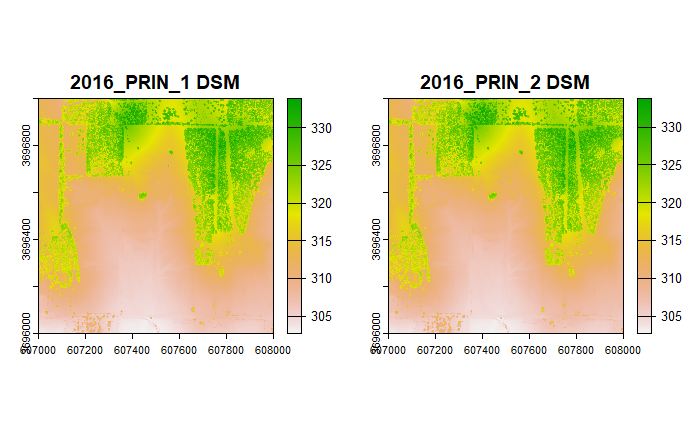
# Plot the DSMs from the 1st and 2nd collections

plot(dsm1, main = "2016_PRIN_1 DSM")

plot(dsm2, main = "2016_PRIN_2 DSM")

# Reset the plotting area

par(mfrow = c(1, 2))



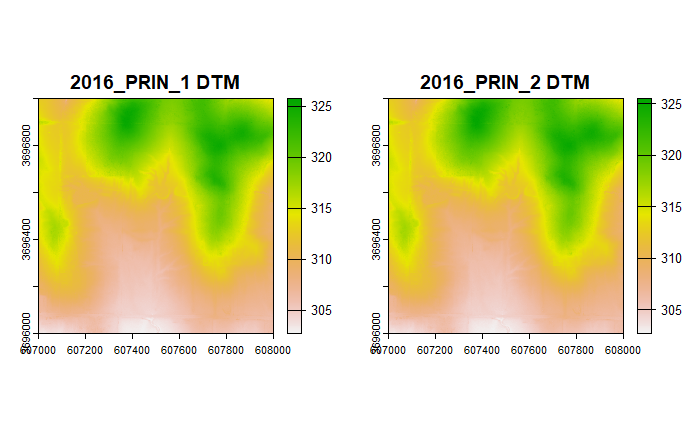
# Plot the DTMs from the 1st and 2nd collections

plot(dtm1, main = "2016_PRIN_1 DTM")

plot(dtm2, main = "2016_PRIN_2 DTM")

Since we want to know what changed between the two days, we will difference the sets of rasters (i.e. DSM1 - DSM2)

# Difference the 2 DSM rasters

dsm_diff <- dsm1 - dsm2



# Calculate mean and standard deviation

dsm_diff_mean <- as.numeric(global(dsm_diff, fun = "mean", na.rm = TRUE))

dsm_diff_std_dev <- as.numeric(global(dsm_diff, fun = "sd", na.rm = TRUE))



# Print the statistics

print(paste("Mean DSM Difference:", round(dsm_diff_mean,3)))

## [1] "Mean DSM Difference: 0.019"

print(paste("Standard Deviation of DSM Difference:", round(dsm_diff_std_dev,3)))

## [1] "Standard Deviation of DSM Difference: 0.743"

The mean is close to zero (0.019 m), indicating there was very little systematic bias between the two days. However, we notice that the standard deviation of the data is quite high at 0.743 meters. Generally we expect NEON LiDAR data to have an error below 0.15 meters! Let's take a look at a histogram of the DSM difference raster to see if we can get a better idea of what's going on.

# Set options to avoid scientific notation

options(scipen = 999)



# Plot a histogram of the raster values

hist(dsm_diff, breaks = 100, main = "Histogram of DSM Difference", xlab = "Height Difference (m)", ylab = "Frequency", col = "lightblue", border = "black")

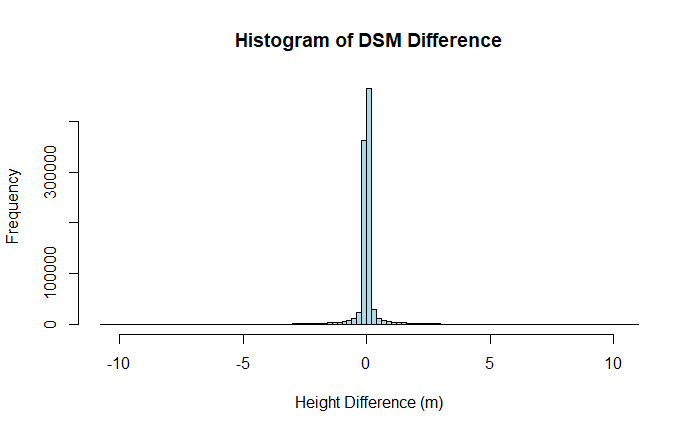
The histogram has long tails, obscuring the distribution near the center. To constrain the x-limits of the histogram we will use the mean and standard deviation just calculated. Since the data appears to be normally distributed, we can constrain the histogram to 95% of the data by including 2 standard deviations above and below the mean.

# Calculate x-axis limits: mean ± 2 * standard deviation

xlim_lower <- dsm_diff_mean - 2 * dsm_diff_std_dev

xlim_upper <- dsm_diff_mean + 2 * dsm_diff_std_dev



# Plot a histogram of the raster values with 100 bins, x-axis set to ±2 standard deviations

hist(dsm_diff, breaks = 250, xlim = c(xlim_lower, xlim_upper), 
     main = "Histogram of Difference DSM", xlab = "Height Difference (m)", 
     ylab = "Frequency", col = "lightblue", border = "black")

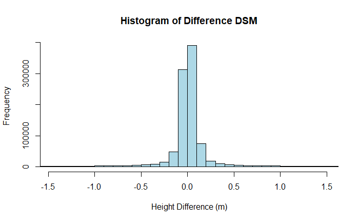
The histogram shows a wide variation in DSM differences, with those at the 95% limit at around +/- 1.5 m. Let's take a look at the spatial distribution of the errors by plotting a map of the difference between the two DSMs. Here we'll also use the extra variable in the plot function to constrain the limits of the colorbar to 95% of the observations.

custom_palette <- colorRampPalette(c("blue", "white", "red"))(9)

breaks = c(-1.75, -1.25, -0.75, -0.25, 0.25, 0.75, 1.25, 2)



# Plot using terra's plot function

plot(dsm_diff, 
     main = "DSM Difference Map", 
     col=custom_palette,
     breaks=breaks,
     axes = TRUE, 
     legend = TRUE)

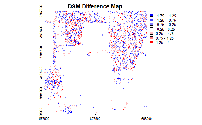
It looks like there is a spatial pattern in the distribution of errors. Now let's take a look at the statistics (mean, standard deviation), histogram and map for the difference in DTMs.

# Difference the 2 DTM rasters

dtm_diff <- dtm1 - dtm2



# Calculate mean and standard deviation

dtm_diff_mean <- as.numeric(global(dtm_diff, fun = "mean", na.rm = TRUE))

dtm_diff_std_dev <- as.numeric(global(dtm_diff, fun = "sd", na.rm = TRUE))



# Print the statistics

print(paste("Mean DTM Difference:", round(dtm_diff_mean,3)))

## [1] "Mean DTM Difference: 0.014"

print(paste("Standard Deviation of DSM Difference:", round(dtm_diff_std_dev,3)))

## [1] "Standard Deviation of DSM Difference: 0.102"


custom_palette <- colorRampPalette(c("blue", "white", "red"))(5)

breaks = c(-1, -0.6, -0.2, 0.2, 0.6, 1)



plot(dtm_diff, 
     main = "DTM Difference Map", 
     col=custom_palette,
     breaks=breaks,
     axes = TRUE, 
     legend = TRUE)

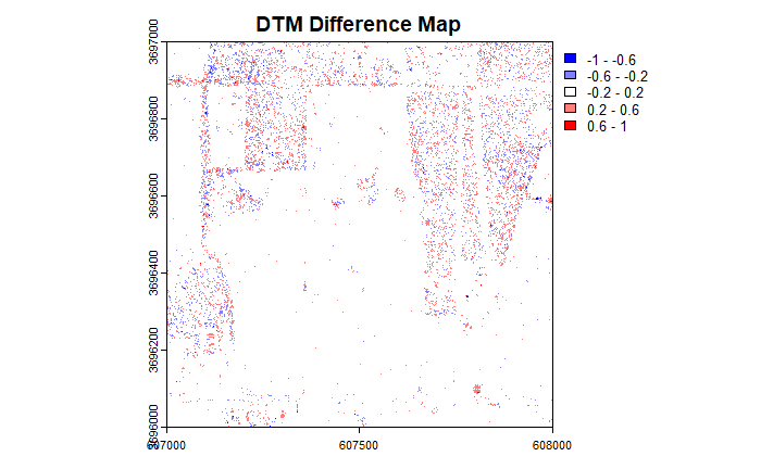
The overall magnitude of differences are smaller than in the DSM but the same spatial pattern of the error is evident.

Now, we'll plot the Canopy Height Model (CHM) of the same area. In the CHM, the tree heights above ground are represented, with all ground pixels having zero elevation. This time we'll use a colorbar which shows the ground as light green and the highest vegetation as dark green.

# Reset the plotting area

par(mfrow = c(1, 2))



# Plot the CHMs from the 1st and 2nd collections

plot(chm1, main = "2016_PRIN_1 CHM")

plot(chm2, main = "2016_PRIN_2 CHM")

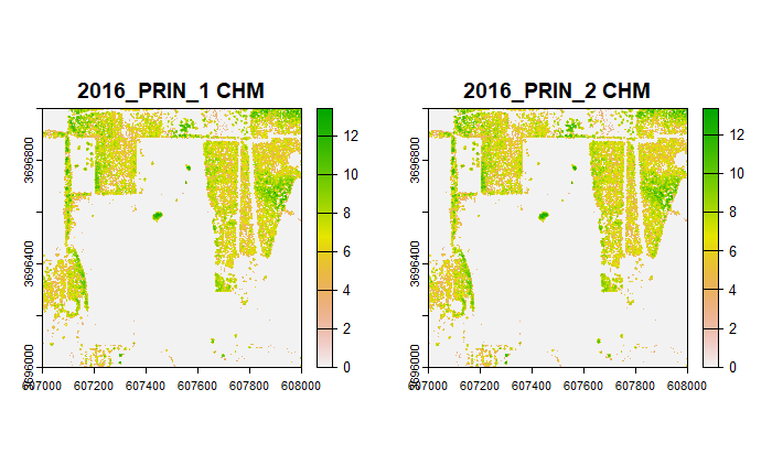
From the CHM, it appears the spatial distribution of error patterns follow the location of vegetation.

Now let's isolate only the pixels in the difference DSM that correspond to vegetation location, calculate the mean and standard deviation, and plot the associated histogram. Before displaying the histogram, we'll remove the no data values from the difference DSM and the non-zero pixels from the CHM.

# Create a mask of non-zero values in the CHM raster

chm_mask <- chm1 != 0



# Apply the veg mask to the DSM difference raster

dsm_diff_masked_veg <- mask(dsm_diff, chm_mask, maskvalue = FALSE)



# Calculate mean and standard deviation of the DSM difference only using vegetated pixels

dsm_diff_masked_veg_mean <- as.numeric(global(dsm_diff_masked_veg, fun = "mean", na.rm = TRUE))

dsm_diff_masked_veg_std_dev <- as.numeric(global(dsm_diff_masked_veg, fun = "sd", na.rm = TRUE))



# Print the statistics

print(paste("Mean DSM Difference on Veg Pixels:", round(dsm_diff_masked_veg_mean,3)))

## [1] "Mean DSM Difference on Veg Pixels: 0.072"

print(paste("Standard Deviation of DSM Difference on Veg Pixels:", round(dsm_diff_masked_veg_std_dev,3)))

## [1] "Standard Deviation of DSM Difference on Veg Pixels: 1.405"


# Calculate x-axis limits: mean ± 2 * standard deviation

masked_xlim_lower <- dsm_diff_masked_veg_mean - 2 * dsm_diff_masked_veg_std_dev

masked_xlim_upper <- dsm_diff_masked_veg_mean + 2 * dsm_diff_masked_veg_std_dev



# Plot a histogram of the raster values with 100 bins, x-axis set to ±2 standard deviations

hist(dsm_diff_masked_veg, breaks = 250, xlim = c(masked_xlim_lower, masked_xlim_upper), 
     main = "Histogram of Difference DSM in Vegetated Areas", xlab = "Height Difference (m)", 
     ylab = "Frequency", col = "lightblue", border = "black")

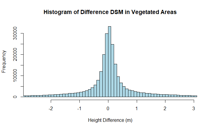
The results show a similar mean difference of near zero, but an extremely high standard deviation of 1.381 m! Since the DSM represents the top of the tree canopy, this provides the level of uncertainty we can expect in the canopy height in forests characteristic of the PRIN site using NEON lidar data.

Next we'll calculate the statistics and plot the histogram of the DTM vegetated areas.

# Apply the veg mask to the DTM difference raster

dtm_diff_masked_veg <- mask(dtm_diff, chm_mask, maskvalue = FALSE)



# Calculate mean and standard deviation of the dtm difference only using vegetated pixels

dtm_diff_masked_veg_mean <- as.numeric(global(dtm_diff_masked_veg, fun = "mean", na.rm = TRUE))

dtm_diff_masked_veg_std_dev <- as.numeric(global(dtm_diff_masked_veg, fun = "sd", na.rm = TRUE))



# Print the statistics

print(paste("Mean DTM Difference on Veg Pixels:", round(dtm_diff_masked_veg_mean,3)))

## [1] "Mean DTM Difference on Veg Pixels: 0.023"

print(paste("Standard Deviation of DTM Difference on Veg Pixels:", round(dtm_diff_masked_veg_std_dev,3)))

## [1] "Standard Deviation of DTM Difference on Veg Pixels: 0.163"

The mean difference is almost zero (0.023 m), and the variation in less than the DSM variation (0.163 m). Let's look at the histogram.

# Calculate x-axis limits: mean ± 2 * standard deviation

masked_xlim_lower <- dtm_diff_masked_veg_mean - 2 * dtm_diff_masked_veg_std_dev

masked_xlim_upper <- dtm_diff_masked_veg_mean + 2 * dtm_diff_masked_veg_std_dev



# Plot a histogram of the raster values with 100 bins, x-axis set to ±2 standard deviations

hist(dtm_diff_masked_veg, breaks = 250, xlim = c(masked_xlim_lower, masked_xlim_upper), 
     main = "Histogram of Difference DTM in Vegetated Areas", xlab = "Height Difference (m)", 
     ylab = "Frequency", col = "lightblue", border = "black")

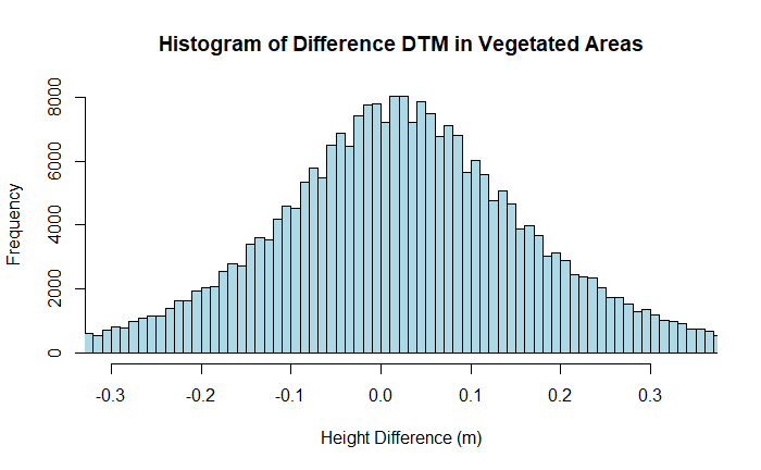
Although the variation of the DTM is lower than in the DSM, it is still larger than expected for lidar. This is because under vegetation there may not be much laser energy reaching the ground, and the points that reach the ground may return with lower signal. The sparsity of points leads to surface interpolation over larger distances, which can miss variations in the topography. Since the distribution of lidar points varied on each day, this resulted in different terrain representations and an uncertainty in the ground surface. This shows that the accuracy of lidar DTMs is reduced when there is vegetation present.

Finally, let's look at the DTM difference on only the ground points (where CHM = 0).

ground_mask <- chm1 == 0



# Apply the ground mask to the DSM difference raster

dsm_diff_masked_ground <- mask(dsm_diff, ground_mask, maskvalue = FALSE)



# Calculate mean and standard deviation of the DSM difference only using vegetated pixels

dsm_diff_masked_ground_mean <- as.numeric(global(dsm_diff_masked_ground, fun = "mean", na.rm = TRUE))

dsm_diff_masked_ground_std_dev <- as.numeric(global(dsm_diff_masked_ground, fun = "sd", na.rm = TRUE))



# Print the statistics

print(paste("Mean DSM Difference on Ground Pixels:", round(dsm_diff_masked_ground_mean,4)))

## [1] "Mean DSM Difference on Ground Pixels: -0.0002"

print(paste("Standard Deviation of DSM Difference on Ground Pixels:", round(dsm_diff_masked_ground_std_dev,3)))

## [1] "Standard Deviation of DSM Difference on Ground Pixels: 0.21"


# Calculate x-axis limits: mean ± 2 * standard deviation

masked_xlim_lower <- dsm_diff_masked_ground_mean - 2 * dsm_diff_masked_ground_std_dev

masked_xlim_upper <- dsm_diff_masked_ground_mean + 2 * dsm_diff_masked_ground_std_dev



# Plot a histogram of the raster values with 100 bins, x-axis set to ±2 standard deviations

hist(dsm_diff_masked_ground, breaks = 500, xlim = c(masked_xlim_lower, masked_xlim_upper), 
     main = "Histogram of Difference DTM over Ground Pixels", xlab = "Height Difference (m)", 
     ylab = "Frequency", col = "lightblue", border = "black")

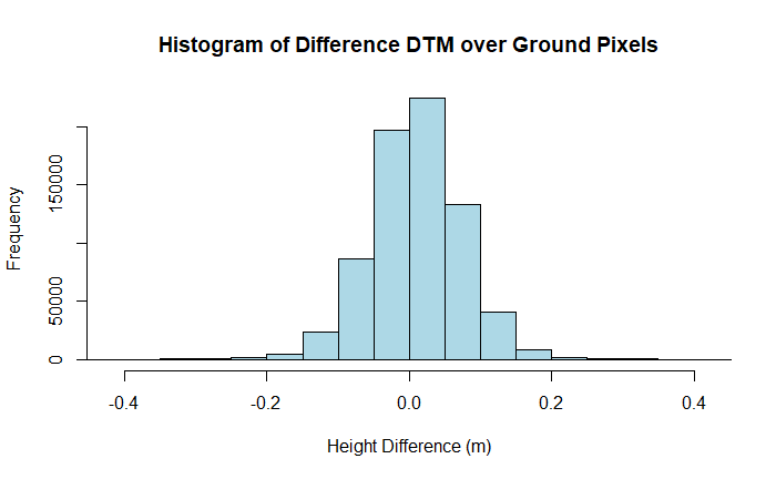
In the open ground scenario we are able to see the error characteristics we expect, with a mean difference of ~ 0 m and a variation of 0.21 m.

This shows that the uncertainty we expect in the NEON lidar system (~0.15 m) is only valid in bare, open, hard-surfaces. We cannot expect the lidar to be as accurate when vegetation is present. Quantifying the top of the canopy is particularly difficult and can lead to uncertainty in excess of 1 m for any given pixel.