AGÕæÈË°Ù¼ÒÀÖ¹Ù·½ÍøÕ¾

This tutorial will walk you through the fundamental principles of working with image raster data in R.

Raster Data

Raster or "gridded" data are data that are saved in pixels. In the spatial world, each pixel represents an area on the Earth's surface. An color image raster is a bit different from other rasters in that it has multiple bands. Each band represents reflectance values for a particular color or spectra of light. If the image is RGB, then the bands are in the red, green and blue portions of the electromagnetic spectrum. These colors together create what we know as a full color image.

Work with Multiple Rasters

In a previous tutorial, we loaded a single raster into R. We made sure we knew the CRS (coordinate reference system) and extent of the dataset among other key metadata attributes. This raster was a Digital Elevation Model so there was only a single raster that represented the ground elevation in each pixel. When we work with color images, there are multiple rasters to represent each band. Here we'll learn to work with multiple rasters together.

Raster Stacks

A raster stack is a collection of raster layers. Each raster layer in the raster stack needs to have the same

• projection (CRS),
• spatial extent and
• resolution.

You might use raster stacks for different reasons. For instance, you might want to group a time series of rasters representing precipitation or temperature into one R object. Or, you might want to create a color images from red, green and blue band derived rasters.

In this tutorial, we will stack three bands from a multi-band image together to create a composite RGB image.

First let's load the R packages that we need: sp and raster.

# load the raster, sp, and rgdal packages
library(raster)
library(sp)
library(rgdal)

# set the working directory to the data
#setwd("pathToDirHere")
wd <- ("~/Git/data/")
setwd(wd)

Next, let's create a raster stack with bands representing

• blue: band 19, 473.8nm
• green: band 34, 548.9nm
• red; band 58, 669.1nm

This can be done by individually assigning each file path as an object.

# import tiffs
band19 <- paste0(wd, "NEON-DS-Field-Site-Spatial-Data/SJER/RGB/band19.tif")
band34 <- paste0(wd, "NEON-DS-Field-Site-Spatial-Data/SJER/RGB/band34.tif")
band58 <- paste0(wd, "NEON-DS-Field-Site-Spatial-Data/SJER/RGB/band58.tif")

# View their attributes to check that they loaded correctly:
band19

## [1] "~/Git/data/NEON-DS-Field-Site-Spatial-Data/SJER/RGB/band19.tif"

band34

## [1] "~/Git/data/NEON-DS-Field-Site-Spatial-Data/SJER/RGB/band34.tif"

band58

## [1] "~/Git/data/NEON-DS-Field-Site-Spatial-Data/SJER/RGB/band58.tif"

Note that if we wanted to create a stack from all the files in a directory (folder) you can easily do this with the list.files() function. We would use full.names=TRUE to ensure that R will store the directory path in our list of rasters.

# create list of files to make raster stack
rasterlist1 <- list.files(paste0(wd,"NEON-DS-Field-Site-Spatial-Data/SJER/RGB", full.names=TRUE))

rasterlist1

## character(0)

Or, if your directory consists of some .tif files and other file types you don't want in your stack, you can ask R to only list those files with a .tif extension.

rasterlist2 <-  list.files(paste0(wd,"NEON-DS-Field-Site-Spatial-Data/SJER/RGB", full.names=TRUE, pattern="tif"))

rasterlist2

## character(0)

Back to creating our raster stack with three bands. We only want three of the bands in the RGB directory and not the fourth band90, so will create the stack from the bands we loaded individually. We do this with the stack() function.

# create raster stack
rgbRaster <- stack(band19,band34,band58)

# example syntax for stack from a list
#rstack1 <- stack(rasterlist1)

This has now created a stack that is three rasters thick. Let's view them.

# check attributes
rgbRaster

## class      : RasterStack 
## dimensions : 502, 477, 239454, 3  (nrow, ncol, ncell, nlayers)
## resolution : 1, 1  (x, y)
## extent     : 256521, 256998, 4112069, 4112571  (xmin, xmax, ymin, ymax)
## crs        : +proj=utm +zone=11 +datum=WGS84 +units=m +no_defs 
## names      : band19, band34, band58 
## min values :     84,    116,    123 
## max values :  13805,  15677,  14343

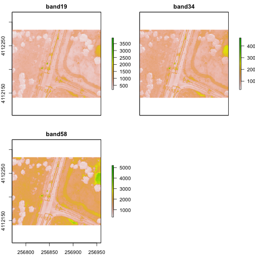
# plot stack
plot(rgbRaster)

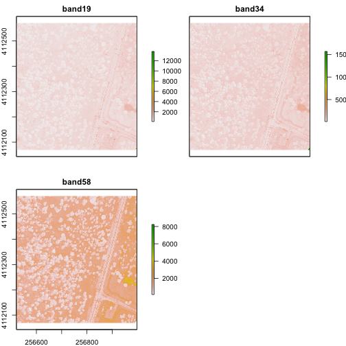
From the attributes we see the CRS, resolution, and extent of all three rasters. The we can see each raster plotted. Notice the different shading between the different bands. This is because the landscape relects in the red, green, and blue spectra differently.

Check out the scale bars. What do they represent?

This reflectance data are radiances corrected for atmospheric effects. The data are typically unitless and ranges from 0-1. NEON Airborne Observation Platform data, where these rasters come from, has a scale factor of 10,000.

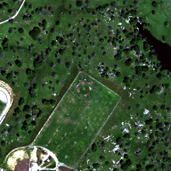
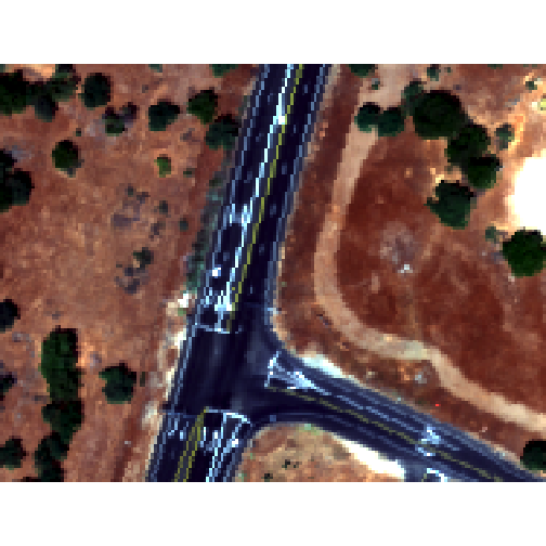
Plot an RGB Image

You can plot a composite RGB image from a raster stack. You need to specify the order of the bands when you do this. In our raster stack, band 19, which is the blue band, is first in the stack, whereas band 58, which is the red band, is last. Thus the order for a RGB image is 3,2,1 to ensure the red band is rendered first as red.

Thinking ahead to next time: If you know you want to create composite RGB images, think about the order of your rasters when you make the stack so the RGB=1,2,3.

We will plot the raster with the rgbRaster() function and the need these following arguments:

• R object to plot
• which layer of the stack is which color
• stretch: allows for increased contrast. Options are "lin" & "hist".

Let's try it.

# plot an RGB version of the stack
plotRGB(rgbRaster,r=3,g=2,b=1, stretch = "lin")

Note: read the raster package documentation for other arguments that can be added (like scale) to improve or modify the image.

Explore Raster Values - Histograms

You can also explore the data. Histograms allow us to view the distrubiton of values in the pixels.

# view histogram of reflectance values for all rasters
hist(rgbRaster)

## Warning in .hist1(raster(x, y[i]), maxpixels = maxpixels, main =
## main[y[i]], : 42% of the raster cells were used. 100000 values used.

## Warning in .hist1(raster(x, y[i]), maxpixels = maxpixels, main =
## main[y[i]], : 42% of the raster cells were used. 100000 values used.

## Warning in .hist1(raster(x, y[i]), maxpixels = maxpixels, main =
## main[y[i]], : 42% of the raster cells were used. 100000 values used.

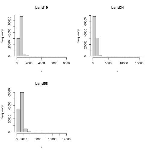
Note about the warning messages: R defaults to only showing the first 100,000 values in the histogram so if you have a large raster you may not be seeing all the values. This saves your from long waits, or crashing R, if you have large datasets.

Crop Rasters

You can crop all rasters within a raster stack the same way you'd do it with a single raster.

# determine the desired extent
rgbCrop <- c(256770.7,256959,4112140,4112284)

# crop to desired extent
rgbRaster_crop <- crop(rgbRaster, rgbCrop)

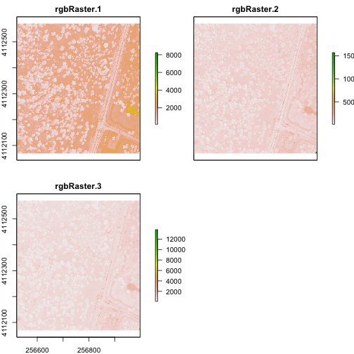
# view cropped stack
plot(rgbRaster_crop)

Raster Bricks in R

In our rgbRaster object we have a list of rasters in a stack. These rasters are all the same extent, CRS and resolution. By creating a raster brick we will create one raster object that contains all of the rasters so that we can use this object to quickly create RGB images. Raster bricks are more efficient objects to use when processing larger datasets. This is because the computer doesn't have to spend energy finding the data - it is contained within the object.

# create raster brick
rgbBrick <- brick(rgbRaster)

# check attributes
rgbBrick

## class      : RasterBrick 
## dimensions : 502, 477, 239454, 3  (nrow, ncol, ncell, nlayers)
## resolution : 1, 1  (x, y)
## extent     : 256521, 256998, 4112069, 4112571  (xmin, xmax, ymin, ymax)
## crs        : +proj=utm +zone=11 +datum=WGS84 +units=m +no_defs 
## source     : memory
## names      : band19, band34, band58 
## min values :     84,    116,    123 
## max values :  13805,  15677,  14343

While the brick might seem similar to the stack (see attributes above), we can see that it's very different when we look at the size of the object.

• the brick contains all of the data stored in one object
• the stack contains links or references to the files stored on your computer

Use object.size() to see the size of an R object.

# view object size
object.size(rgbBrick)

## 5762000 bytes

object.size(rgbRaster)

## 49984 bytes

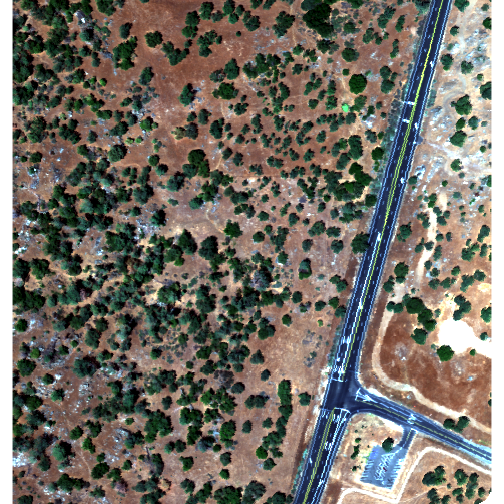
# view raster brick
plotRGB(rgbBrick,r=3,g=2,b=1, stretch = "Lin")

Notice the faster plotting? For a smaller raster like this the difference is slight, but for larger raster it can be considerable.

Write to GeoTIFF

We can write out the raster in GeoTIFF format as well. When we do this it will copy the CRS, extent and resolution information so the data will read properly into a GIS program as well. Note that this writes the raster in the order they are in. In our case, the blue (band 19) is first but most programs expect the red band first (RGB).

One way around this is to generate a new raster stack with the rasters in the proper order - red, green and blue format. Or, just always create your stacks R->G->B to start!!!

# Make a new stack in the order we want the data in 
orderRGBstack <- stack(rgbRaster$band58,rgbRaster$band34,rgbRaster$band19)

# write the geotiff
# change overwrite=TRUE to FALSE if you want to make sure you don't overwrite your files!
writeRaster(orderRGBstack,paste0(wd,"NEON-DS-Field-Site-Spatial-Data/SJER/RGB/rgbRaster.tif"),"GTiff", overwrite=TRUE)

Import A Multi-Band Image into R

You can import a multi-band image into R too. To do this, you import the file as a stack rather than a raster (which brings in just one band). Let's import the raster than we just created above.

# import multi-band raster as stack
multiRasterS <- stack(paste0(wd,"NEON-DS-Field-Site-Spatial-Data/SJER/RGB/rgbRaster.tif")) 

# import multi-band raster direct to brick
multiRasterB <- brick(paste0(wd,"NEON-DS-Field-Site-Spatial-Data/SJER/RGB/rgbRaster.tif")) 

# view raster
plot(multiRasterB)

plotRGB(multiRasterB,r=1,g=2,b=3, stretch="lin")