Tutorial
Intro to AOP Datasets in Google Earth Engine (GEE) using Python
Last Updated: Aug 19, 2024
Objectives
After completing this tutorial, you will be able to use Python to:
- Determine the available AOP datasets in Google Earth Engine
- Read in and visualize AOP Reflectance, RGB Camera, and Lidar raster datasets
- Become familiar with the AOP Image Properties
- Filter data based off image properties to pull in dataset(s) of interest
- Explore the interactive mapping features in
geemap
Requirements
To follow along with this code, you will need to:
- Sign up for a non-commercial Google Earth Engine account here .
- Install Python 3.9+
- Install required Python packages
-
pip install earthengine-api --upgrade -
pip install geemap
You may need to run the following to upgrade the google-api-python-client:
-
pip install --upgrade google-api-python-client
Notes:
- This tutorial was developed using Python 3.9, so if you are installing Python for the first time, we recommend that version or higher. This lesson was written in Jupyter Notebook so you can run each cell chunk individually, but you can also use a different IDE (Interactive Development Environment) of your choice.
- If not using Jupyter, we recommend using Spyder, which has similar functionality. You can install both Python, Jupyter Notebooks, and Spyder by downloading .
Additional Resources
AOP data in Google Earth Engine
is a platform for carrying out continental and planetary scale geospatial analyses. It has a multi-pedabyte catalog of satellite imagery and geospatial datasets, and is a powerful environment for comparing and scaling up NEON airborne datasets.
The NEON data products that have been made available on GEE can be currently be accessed through the projects/neon-prod-earthengine folder with an appended suffix of the dataset Acronym and Revision Number, shown in the table below.
| Acronym | Revision | Data Product | Data Product ID |
|---|---|---|---|
| HSI_REFL | 001 | Surface Directional Reflectance | |
| HSI_REFL | 002 | Surface Bidirectional Reflectance | |
| RGB | 001 | Red Green Blue (Camera Imagery) | |
| DEM | 001 | Digital Surface and Terrain Models (DSM/DTM) | |
| CHM | 001 | Ecosystem Structure (Canopy Height Model; CHM) |
To access the NEON AOP data you can read in the Image Collection ee.ImageCollection followed by the path, eg. the Surface Directional Reflectance can be found under the path projects/neon-prod-earthengine/assets/HSI_REFL/001. You can then filter down to a particular site and year of interest using the properties.
First, import the relevant Earth Engine Python packages, earthengine-api and . This lesson was written using geemap version 0.22.1. If you have an older version installed, used the command below to update.
GEE Python Package Installation and Authentication
import ee, geemap
In order to use Earth Engine from within this Jupyter Notebook, we need to first Authenticate (which requires generating a token) and then Initialize, as below. For more detailed instructions on the Authentication process, please refer to the: .
geemap.__version__
'0.22.1'
ee.Authenticate()
To authorize access needed by Earth Engine, open the link that pops up and follow the prompts which will generate a token.
The authorization workflow will generate a code, which you should paste in the box below.

Copy the token into the box, and when you hit enter, you should receive the notice: "Successfully saved authorization token."
ee.Initialize()
Now that you've Authenticated and Initialized your Earth Engine account, you can start using the Python API to interact with GEE using the ee and geemap packages.
First let's read in the Surface Directional Reflectance Image Collection (HSI_REFL/001) and see what data are available in GEE.
# Read in the NEON AOP Surface Directional Reflectance Collection:
refl001 = ee.ImageCollection('projects/neon-prod-earthengine/assets/HSI_REFL/001')

# Count and list all available sites in the NEON directional reflectance image collection:
# Get the number of reflectance images
refl001_count = refl001.size()
refl001_count = str(refl001_count.getInfo())
print(f'Found {refl001_count} NEON Directional Reflectance Images in GEE')

refl001_year_sites = refl001.aggregate_array('system:index').getInfo()
print('\nLast 10 reflectance datasets available:')
print(refl001_year_sites[-10:])
Found 48 NEON Directional Reflectance Images in GEE

Last 10 reflectance datasets available:
['2021_GRSM_5', '2021_HEAL_4', '2021_JERC_6', '2021_JORN_4', '2021_MCRA_2', '2021_OAES_5', '2021_OSBS_6', '2021_SJER_5', '2021_SOAP_5', '2021_SRER_4']
We can also look for data for a specified site - for example look at all the years of AOP reflectance (001) data available for a given site.
# See the years of data available for the specified site:
site = 'CPER'

# Get the flight year and site information
flight_years = refl001.aggregate_array('FLIGHT_YEAR').getInfo()
sites = refl001.aggregate_array('NEON_SITE').getInfo()

print('\nYears of Directional Reflectance data available in GEE for ',site+':')
print([year_site[0] for year_site in zip(flight_years,sites) if site in year_site])
Years of Directional Reflectance data available in GEE for  CPER:
[2013, 2017, 2020, 2020, 2021]
Let's take a look at another dataset, the high-resolution RGB camera imagery:
# Read in the NEON AOP Camera (RGB) Collection:
rgb = ee.ImageCollection('projects/neon-prod-earthengine/assets/RGB/001')

# List all available sites in the NEON directional reflectance image collection:
print('Available NEON Camera Images:')
# Get the number of RGB images
rgb_count = rgb.size()
print('Count: ', str(rgb_count.getInfo())+'\n')
print(rgb.aggregate_array('system:index').getInfo())
Available NEON Camera Images:
Count:  44

['2016_HARV_3', '2017_CLBJ_2', '2017_GRSM_3', '2017_SERC_3', '2018_CLBJ_3', '2018_OAES_3', '2018_SRER_2', '2018_TEAK_3', '2019_BART_5', '2019_CLBJ_4', '2019_HARV_6', '2019_HEAL_3', '2019_JORN_3', '2019_OAES_4', '2019_SOAP_4', '2020_CPER_7', '2020_NIWO_4', '2020_RMNP_3', '2020_UKFS_5', '2020_UNDE_4', '2020_YELL_3', '2021_ABBY_4', '2021_BLAN_4', '2021_BONA_4', '2021_CLBJ_5', '2021_DEJU_4', '2021_DELA_6', '2021_HEAL_4', '2021_JERC_6', '2021_JORN_4', '2021_LENO_6', '2021_MLBS_4', '2021_OAES_5', '2021_OSBS_6', '2021_SERC_5', '2021_SJER_5', '2021_SOAP_5', '2021_SRER_4', '2021_TALL_6', '2021_WREF_4', '2022_OAES_6', '2022_UNDE_5', '2023_CLBJ_7', '2023_OAES_7']
Similarly, you can read in the DEM and CHM collections as follows:
# Read in the NEON AOP DEM Collection (this includes the DTM and DSM as 2 bands)
dem = ee.ImageCollection('projects/neon-prod-earthengine/assets/DEM/001')

# Read in the NEON AOP CHM Collection
chm = ee.ImageCollection('projects/neon-prod-earthengine/assets/CHM/001')
Explore Image Properties
Now that we've read in a couple of image collections, let's take a look at some of the image properties using geemap.image_props:
props = geemap.image_props(refl001.first())

# Display the property names for the first 15 properties:
props.keys().getInfo()[:16]

# Optionally display all properties by uncommenting the line below
# props
['AOP_VISIT_NUMBER',
 'DESCRIPTION',
 'FLIGHT_YEAR',
 'IMAGE_DATE',
 'NEON_DATA_PROD_ID',
 'NEON_DATA_PROD_URL',
 'NEON_DOMAIN',
 'NEON_SITE',
 'NOMINAL_SCALE',
 'PROVISIONAL_RELEASED',
 'RELEASE_YEAR',
 'SCALE_FACTOR',
 'SENSOR_NAME',
 'SENSOR_NUMBER',
 'WL_FWHM_B001',
 'WL_FWHM_B002']
You can also look at all the Image properties by typing props. This generates a long output, so we will just show a portion of the output from that:
AOP_VISIT_NUMBER: 1
DESCRIPTION :Orthorectified surface directional reflectance (0-1 unitless, scaled by 10000) ...
FLIGHT_YEAR: 2013
IMAGE_DATE: 2013-06-25
NEON_DATA_PROD_ID: DP3.30006.001
NEON_DATA_PROD_URL: https://data.neonscience.org/data-products/DP3.30006.001
NEON_DOMAIN: D10
NEON_SITE: CPER
NOMINAL_SCALE: 1
PROVISIONAL_RELEASED: RELEASED
RELEASE_YEAR :2024R
SCALING_FACTOR:10000
SENSOR_NAME: AVIRIS-NG
SENSOR_NUMBER: NIS1
WL_FWHM_B001: 382.3465,5.8456

system:asset_size: 68059.439009 MB
system:band_names: List (442 elements)
system:id: projects/neon-prod-earthengine/assets/HSI_REFL/001/2013_CPER_1
system:index: 2013_CPER_1
system:time_end: 2013-06-25 10:42:05
system:time_start: 2013-06-25 08:30:45
system:version: 1689911980211725
The image properties contain some additional relevant information about the dataset, and are variables you can filter on to select a subset of the data. A lot of these properties are self-explanatory, but some of them may be less apparent. A short description of a few properties is outlined below. Note that when the datasets become part of the Google Public Datasets, you will be able to see descriptions of the properties in GEE
-
PROVISIONAL_RELEASED: Whether the data are available provisionally, or are Released. See /data-samples/data-management/data-revisions-releases for more information on the NEON release process. -
RELEASE_YEAR: The year of the release tag, if the data have been Released. -
SENSOR_NAME: The name of the hyperspectral sensor. All NEON sensors are JPL AVIRIS-NG sensors. -
SENSOR_NUMBER: The payload number, NIS1 = NEON Imaging Spectrometer, Payload 1. NEON Operates 3 separate payloads, each with a unique hyperspectral sensor (as well as unique LiDAR and Camera sensors). -
WL_FWHM_B###: Center Wavelength (WL) and Full Width Half Max (FWHM) of the band, both in nm.
In addition, there are some system properties, including information about the size of the asset, the band names (most of these are just band numbers but the QA bands have more descriptive names), as well as the start and end time of the collection.
Filter an Image Collection
One of the most useful features of working with AOP data ingested in Earth Engine is the ability to filter by properties, such as the site name, dates, etc. In this next section, we will show how to filter datasets to extract only data of interest. We'll use the NEON's Harvard Forest (HARV), in Massachusettes.
# See the years of data available for a specified site:
site = 'HARV'

# Get the flight year and site information
rgb_flight_years = rgb.aggregate_array('FLIGHT_YEAR').getInfo()
rgb_sites = rgb.aggregate_array('NEON_SITE').getInfo()

print('\nYears of RGB data available in GEE for',site+':')
print([year_site[0] for year_site in zip(rgb_flight_years, rgb_sites) if site in year_site])
Years of RGB data available in GEE for HARV:
[2016, 2019]
# Get the flight year and site information
refl001_flight_years = refl001.aggregate_array('FLIGHT_YEAR').getInfo()
refl001_sites = refl001.aggregate_array('NEON_SITE').getInfo()

print('\nYears of Directional Reflectance data available in GEE for',site+':')
print([year_site[0] for year_site in zip(refl001_flight_years, refl001_sites) if site in year_site])
Years of Directional Reflectance data available in GEE for HARV:
[2014, 2016, 2017, 2018, 2019]
# Specify the start and end dates
year = 2019
start_date2019 = ee.Date.fromYMD(year, 1, 1)
end_date2019 = start_date2019.advance(1, "year")

# Filter the RGB image collection on the site and dates
harv_rgb2019 = rgb.filterDate(start_date2019, end_date2019).filterMetadata('NEON_SITE', 'equals', site).mosaic()
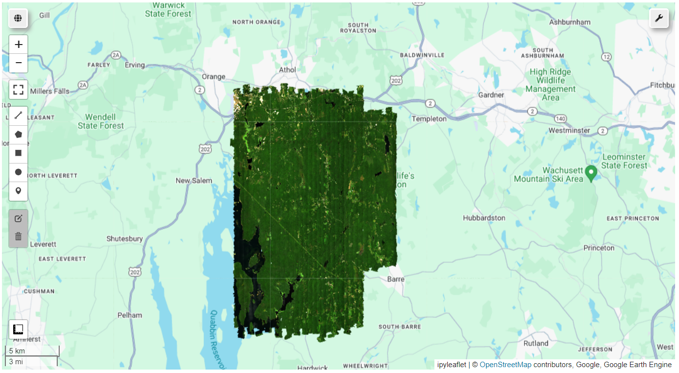
Add Data Layers to the Map
In order to visualize and interact with the dataset, we can use geemap.Map() as follows, to display Harvard Forest camera and directional reflectance imagery from 2019.
Map = geemap.Map()

# Specify center location of HARV
# NEON field site information can be found on the NEON website here > /field-sites/harv
geo = ee.Geometry.Point([-72.17, 42.5])

# Set the visualization parameters so contrast is maximized
rgb_vis_params = {'min': 45, 'max': 200, 'gamma': .6}

# Add the RGB data as a layer to the Map
Map.addLayer(harv_rgb2019, rgb_vis_params, 'HARV 2019 RGB Camera');

# Center the map on the site center and set zoom level
Map.centerObject(geo, 11);

Map
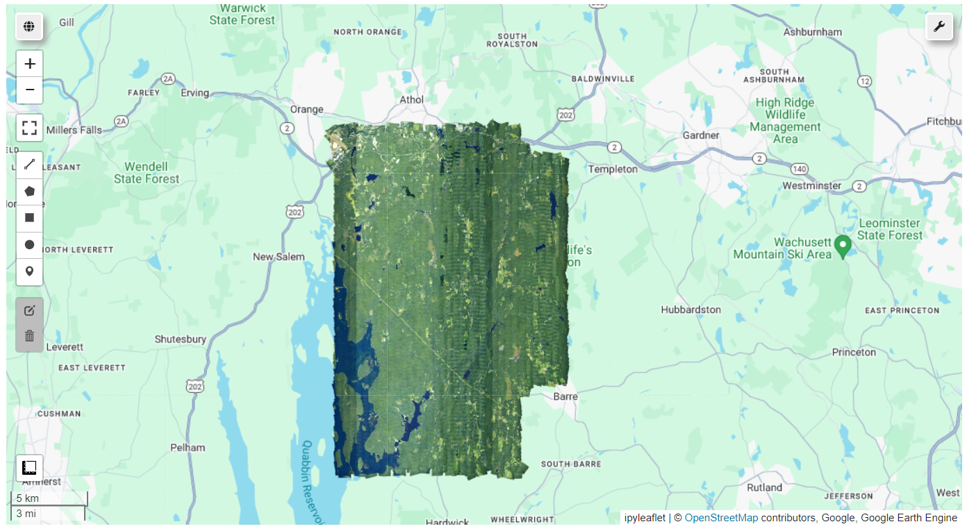
Surface Directional Reflectance
Next let's take a look at one of the Surface Directional Reflectance datasets. We will pull in only the data bands, for this example.
Reflectance Data Bands
Map = geemap.Map()

# Read in the first image of the Reflectance Image Collection
harv_refl2019 = refl001.filterDate(start_date2019, end_date2019).filterMetadata('NEON_SITE', 'equals', site).mosaic()

# Read in only the data bands, all of which start with "B", eg. "B001"
harv_refl2019_data = harv_refl2019.select('B.*')

# Set the visualization parameters so contrast is maximized, and display RGB bands (true-color image)
refl001_viz = {'min':0, 'max':1200, 'gamma':0.9, 'bands':['B053','B035','B019']};

# Add the reflectance data as a Layer to the Map
Map.addLayer(harv_refl2019_data, refl001_viz, 'Harvard Forest 2019 Directional Reflectance');

# Center the map on the site center and set zoom level
Map.centerObject(geo, 11);

Map
Reflectance QA Bands
Before we used a regular expression to pull out only the bands starting with "B". We can also take a look at the remaining bands using a similar expression, but this time excluding bands starting with "B". These comprise all of the QA-related bands that provide additional information and context about the data bands. This next chunk of code prints out the IDs of all the QA bands.
# Read in only the QA bands, none of which start with "B"
reflQA_bands = harv_refl2019.select('[^B].*')

# Create a dictionary of the band information
reflQA_band_info = reflQA_bands.getInfo()
type(reflQA_band_info)

# Loop through the band info dictionary to print out the ID of each band
print('QA bands:\n')
for i in range(len(reflQA_band_info['bands'])):
    print(reflQA_band_info['bands'][i]['id'])
QA bands:

Aerosol_Optical_Depth
Aspect
Cast_Shadow
Dark_Dense_Vegetation_Classification
Haze_Cloud_Water_Map
Illumination_Factor
Path_Length
Sky_View_Factor
Slope
Smooth_Surface_Elevation
Visibility_Index_Map
Water_Vapor_Column
to-sensor_Azimuth_Angle
to-sensor_Zenith_Angle
Weather_Quality_Indicator
Acquisition_Date
Most of these QA bands are related to the Atmospheric Correction (ATCOR), one of the spectrometer processing steps which converts Radiance to Reflectance. For more details on this process, NEON provides an Algorithm Theoretical Basis Document (ATBD), which is available on the NEON data portal and linked here: .
The Weather_Quality_Indicator is particularly useful for assessing data quality. The weather quality indicator includes information about the cloud conditions during the flight, as reported by the flight operators, where 1 corresponds to <10% cloud cover, 2 corresponds to 10-50% cloud cover, and 3 corresponds to >50% cloud cover. We recommend using only clear-sky data (1) for a typical analysis, as it results in the highest quality reflectance data.
You may also be interested in the Acquisition_Date if, for example, you are linking field data collected on a specific date, or are interested in finding satellite data collected close in time to the AOP imagery.
The next chunks of code show how to add the Weather QA bands to the Map Layer.
Weather Quality Indicator Band
Map = geemap.Map()

harv_refl_weather_qa2019 = harv_refl2019.select(['Weather_Quality_Indicator']);

# Define a palette for the weather - to match NEON AOP's weather color conventions (green-yellow-red)
gyr_palette = ['green','yellow','red']

# Visualization parameters to display the weather bands (cloud conditions) with the green-yellow-red palette
weather_viz = {'min': 1, 'max': 3, 'palette': gyr_palette, 'opacity': 0.3};

# Add the RGB data as a layer to the Map
Map.addLayer(harv_refl_weather_qa2019, weather_viz, 'HARV 2019 Weather QA');

# Center the map on the site center and set zoom level
Map.centerObject(geo, 11);

Map
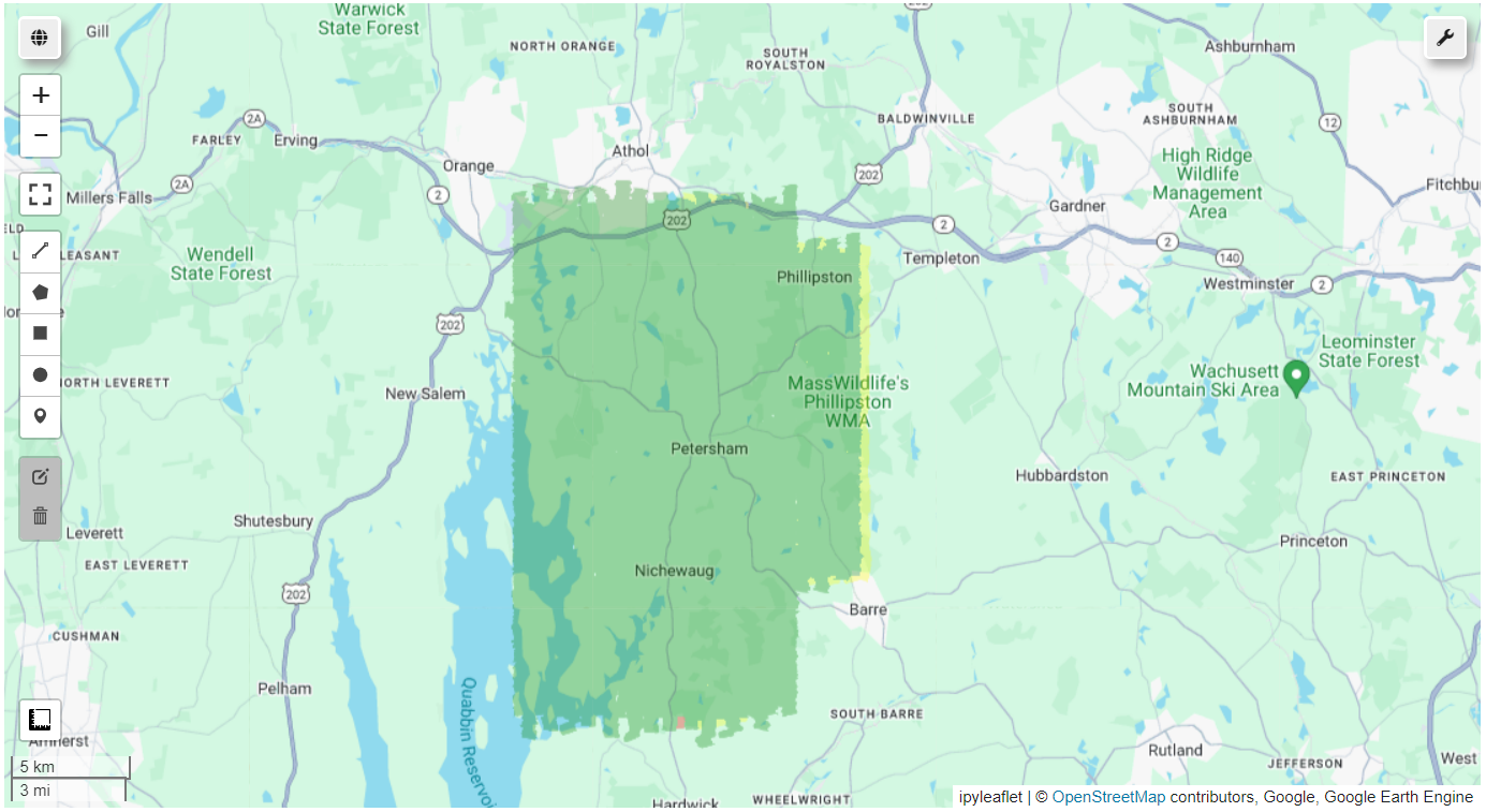
In 2019, the AOP was able to collect all but the easternmost flightline in green, or clear-sky weather conditions. Let's take a look at the data from 2018 for comparison:
# Specify the start and end dates
year = 2018
start_date2018 = ee.Date.fromYMD(year, 1, 1)
end_date2018 = start_date2018.advance(1, "year")

# Filter the reflectance image collection on the site and dates
harv_refl2018 = refl001.filterDate(start_date2018, end_date2018).filterMetadata('NEON_SITE', 'equals', site).mosaic()

Map = geemap.Map()

harv_refl_weather_qa2018 = harv_refl2018.select(['Weather_Quality_Indicator']);

# Define a palette for the weather - to match NEON AOP's weather color conventions (green-yellow-red)
gyr_palette = ['green','yellow','red']

# Visualization parameters to display the weather bands (cloud conditions) with the green-yellow-red palette
weather_viz = {'min': 1, 'max': 3, 'palette': gyr_palette, 'opacity': 0.3};

# Add the weather QA layer to the map
Map.addLayer(harv_refl_weather_qa2018, weather_viz, 'HARV 2019 Weather QA');

# Center the map on the site center and set zoom level
Map.centerObject(geo, 11);

Map
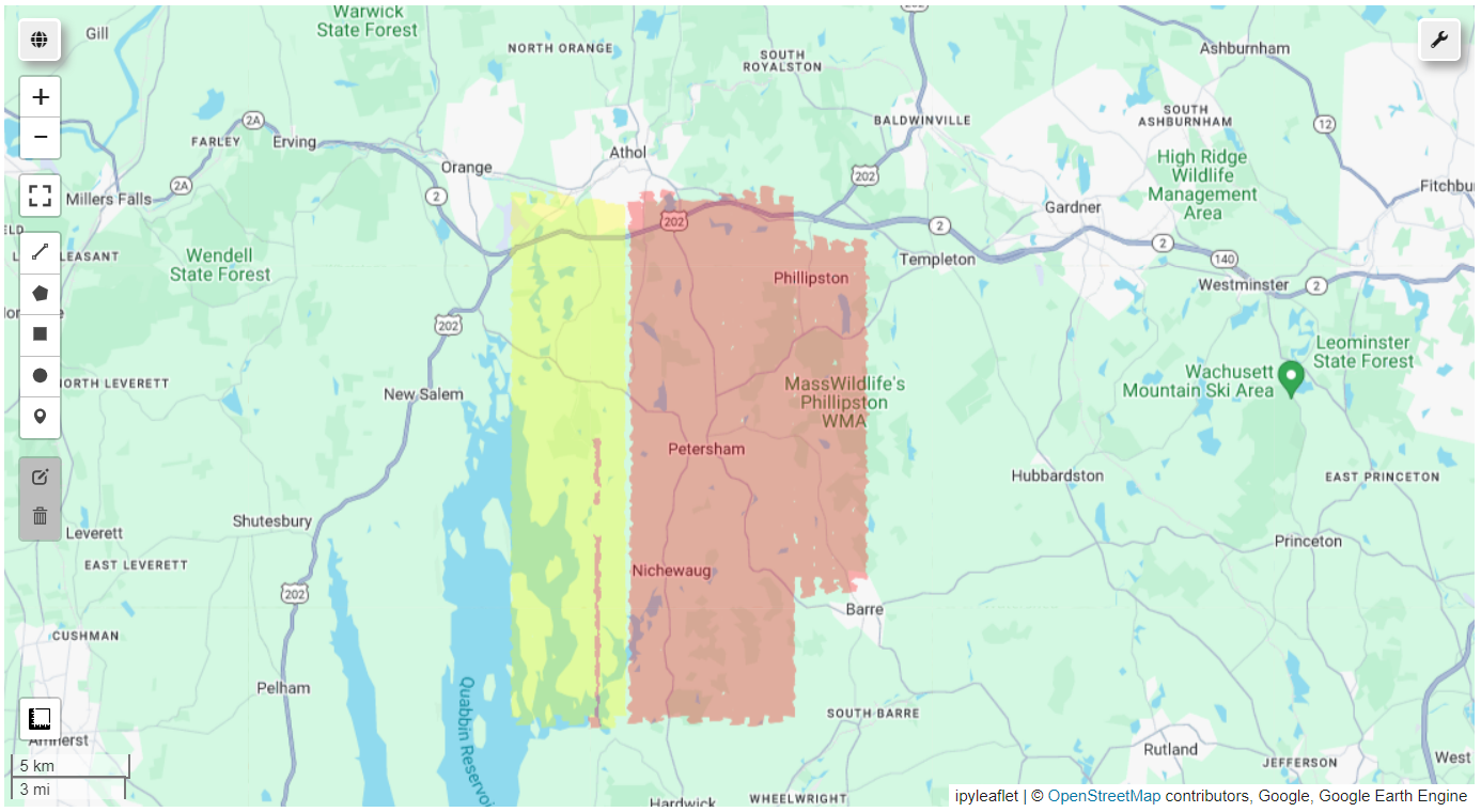
We can see that in 2019, the weather conditions were sub-optimal for collecting. When working with the AOP data, this is important information to keep in mind - as the reflectance data (and other optical data, such as the camera data) collected in cloudy sky conditions are not directly comparable to data collected in clear skies.
Recap
In this lesson, you learned how to access the five NEON datasets that are available in GEE: Bidirectional Reflectance (HSI_REFL/002), Surface Directional Reflectance (HSI_REFL/001), Camera (RGB/001), and LiDAR-derived Digital Elevation (Terrain and Surface) Models (DEM/001) and Ecosystem Structure / Canopy Height Model (CHM/001). You generated code to determine which AOP datasets are available in GEE for a given Image Collection. You explored the directional reflectance image properties and learned how to filter on metadata to pull out a subset of Images or a single Image from an Image Collection. You learned how to use the geemap package to add data layers to the interactive map panel. And lastly, you learned how to select and visualize the Weather_Quality_Indicator band, which is a useful first step in assessing the data quality of the AOP reflectance and camera imagery.
This is a great starting point for your own research!